Nowadays mobile devices with wireless communication capability are becoming widespread; thereby ad-hoc networks that allow direct communication between devices without access points or base stations is of great interest. Wireless local area network (WLAN) standard IEEE 802.11 [1] defines carrier sense multiple access with collision avoidance (CSMA/CA) as an access method for autonomous decentralized control. As CSMA protocol implements autonomous transmission control, a sender node first performs carrier sense (clear channel assessment [CCA]), then it starts transmission if the channel is idle for a certain period of time, i.e., the DCF interframe space (DIFS) period. If any other nodes are using the channel, it waits until the channel becomes idle, and then waits another DIFS period plus a random back off period before it starts transmission. With this autonomous decentralized control, frame collisions can be avoided. However, there is a problem in that the sender node cannot know the channel usage condition of nodes outside its reception range. If the sender node happens to start trans-mission when one of those nodes outside the reception range is also in transmission, a collision occurs at the receiver node. This is the hidden node problem and degrades the network throughput [2].
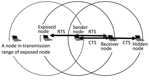
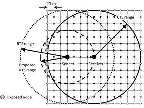
The request to send/clear to send (RTS/CTS) method was introduced in the 802.11 standard to solve this hidden node problem. However, the RTS/CTS method causes a new problem called the exposed node problem. Fig. 1 shows an example of hidden and exposed nodes. In Fig. 1, the Hidden Node is defined as a node located within the receive range of the Receiver Node but outside the transmission range of the Sender Node. In Fig. 1, we assume that transmission range and receive range are equal. The Exposed Node is defined as a node located within the transmission range of the Sender Node but outside the transmission range of the Receiver Node.
CTS solves the hidden node problem while RTS causes the exposed node problem as follows. As the exposed nodes receive RTS from the sender, they must hold their transmissions. This allows the sender to receive CTS and ACK from the receiver without collisions, during this time the exposed nodes cannot transmit to any other nodes during that network allocation vector (NAV) period defined in the RTS frame, and their throughput degrades substantially [3, 4]. Holding transmission for the entire NAV period is an unnecessarily large penalty because when the sender is in transmission mode it cannot receive anything from the exposed nodes. Thereby the exposed node should be allowed to transmit when the sender node is sending data frames. The exposed nodes need to hold their transmission only when the sender receives the CTS and ACK frames, and these take a relatively short period compared to the data frame transmission period. In Fig. 1, the Exposed Node should be able to send frames to a node in its transmission range when the Sender Node is sending a data frame to the Receiver Node. In this paper we propose an asymmetric RTS/CTS method to reduce the number of exposed nodes. The asymmetric RTS/CTS method assigns asymmetric transmission rates to the RTS and CTS. This method controls the transmission range of RTS and reduces the number of exposed nodes to prevent throughput degradation. Experimental results by simulation shows that the proposed method improves the entire network throughput compared to the standard RTS/CTS method, and also helps to equalize variation of the throughput among each node.
This paper is organized as follows. In Section Ⅱ, existing research related to exposed nodes and their drawbacks are reviewed. In Section Ⅲ, the standard RTS/CTS method is explained. In Section Ⅳ, our proposed asymmetric RTS/CTS method is explained. In Section Ⅴ, the computer simulation and its result are used to show the effectiveness of the proposed method. In Section Ⅵ, we summarize this paper and future research directions are discussed.
In this section, we review related research of exposed nodes and mention their drawbacks. In [4], the following method is proposed. A node can recognize itself as an exposed node by receiving RTS not destined for it, not receiving the corresponding CTS, and receiving DATA from the RTS sender. Then the exposed node can send its data frame in parallel during the data frame transmission period of the sender node. This method is improved and named P-MAC in [5]. P-MAC involves a more sophisticated way to avoid collision by introducing ‘interference range’. These are interesting approaches to utilize the fact that transmission of an exposed node does not cause collisions or interference as long as the sender node is in transmission state. In these methods, transmissions of exposed nodes must be carefully synchronized to DATA from the sender node, and it must complete the transmission before the DATA transmission is complete. P-MAC has also been modified to send ACK at random intervals, which is a deviation from the standard protocol. Our proposed method exploits this same fact without modifying protocol and maintains complete compatibility with the standard method. In [6, 7], the following method is proposed. Each node in the network knows the locations of all other nodes in a database beforehand and knows which nodes are exposed nodes. A sender node notifies the exposed nodes which can send data frames in parallel, the same as in [4, 5], and lets them send data frames. This method may not work well on a large scale and with mobile nodes. In [8], to eliminate exposed nodes, selective disregard of NAVs (SDN) is proposed. This selectively ignores certain physical carrier sense and NAVs. Modification to physical layer and CTS frame is required to perform this operation. This method needs additional functionalities to be implemented in all nodes and lacks compatibility with the IEEE standard. There are some studies [9-11] which assume different transmission rate for the RTS/CTS frame and data frame, but no studies assume different transmission rate for the RTS and CTS frames. Our proposed method does not need exposed nodes to adjust their transmissions. We only need to adjust the transmission rate of the RTS and CTS in an asymmetric fashion.
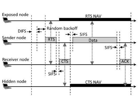
In this section we explain the RTS/CTS method defined by the WLAN standard IEEE 802.11. Fig. 2 shows the standard RTS/CTS method in the case of four nodes, i.e., the Exposed Node, Sender Node, Receiver Node, and Hidden Node. The standard RTS/CTS method is called ‘four-way handshaking’ and is outlined below.
1) A sender node performs carrier sense and sends RTS. If the cannel is busy the sender node waits until the channel becomes idle, it waits a further DIFS period plus a random back off period before its transmission. At this moment, the exposed nodes also receive RTS. The exposed nodes must hold their transmissions for the NAV period as must all other nodes which received the RTS frame.2) The receiver node receives the RTS and sends CTS to the sender node after the short interframe space (SIFS) period. At this moment, hidden nodes also receive the CTS. The hidden nodes must hold their transmissions for the NAV period as must all other nodes which received the CTS.3) The sender node receives the CTS and sends the data frame to the receiver node after the SIFS period.4) The receiver node receives the data frame and sends ACK (Acknowledgement) back to the sender node after the SIFS period.
This mechanism was introduced with the first version of the IEEE 802.11 standard in 1997. At that time, available transmission rates were only 1 Mbps and 2 Mbps. The standard defines that control frames, such as the RTS/CTS/ACK, should be sent at one of the basic data rates in order to be received by as many nodes as possible.
Though it mitigates the hidden node problem, RTS/ CTS itself can be an overhead. In [12], it is reported that in a multi-rate environment with an auto rate fallback, such as in the 802.11a infrastructure mode network, RTS/ CTS should be always enabled for highly loaded networks. Even if there are no hidden nodes, aggregate throughput is better with RTS/CTS when the data frame size is larger than 640 bytes (aggregate throughput is roughly 40% better at 1000 bytes). This is due to fewer collisions as the channel is reserved by a small RTS frame and occasional collision of RTS frames does not cause auto rate fallback. Therefore reducing the exposed node problem helps to extend RTS/CTS usage.
Using the standard RTS/CTS method we can avoid collisions at the receiver node by eliminating hidden nodes. However, RTS induces exposed nodes and their transmissions are held for unnecessarily long periods, thereby degrading the entire network throughput. Our proposed method configures RTS and CTS transmission rates asymmetrically and controls the range of these frames in order to reduce the number of exposed nodes.
>
B. Consideration about RTS and CTS Transmission Rate
As in Fig. 2, the Receiver Node is provoked to send CTS by receiving RTS. If the RTS range is set to the minimum distance, only reaching the receiver node, this is enough to provoke CTS from the receiver node.
The RTS transmission rate need not be the basic rate and it can be the same as the transmission rate for the data frame, i.e., this transmission rate should be the maximum rate which the sender and the receiver nodes have agreed to. From Table 1, it can be said that the effective transmission range becomes shorter with higher transmission rates. This means that we can make the effective range the smallest by adjusting the RTS transmission rate to the maximum. CTS should reach to all possible nodes that can cause collisions at the receiver node; thereby data frame reception at the receiver node can be protected. Those possible interfering nodes may transmit at the basic rate or the lowest transmission rate, thus CTS should be sent at the lowest transmission rate as well.
[Table 1.] Relationship between transmission rate and distance
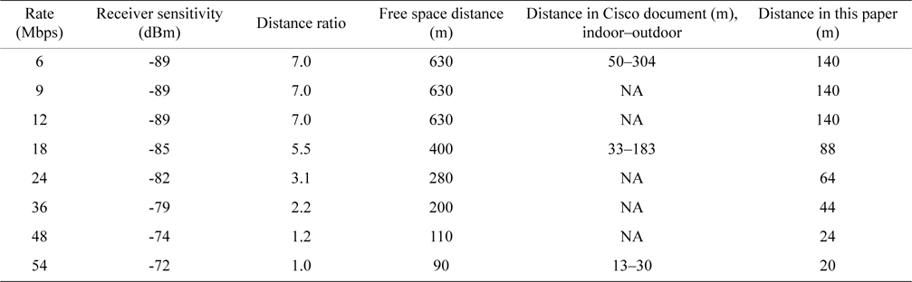
Relationship between transmission rate and distance
Transmission range is not the same as radio range. By transmission range we mean the range at which NAV is correctly interpreted and observed by any receiver node. All IEEE 802.11 frames have PHY layer convergence procedure (PLCP) preamble and header, and these are always transmitted at 6 Mbps (for 802.11a) and this transmission rate cannot be changed. The following parts of the frame, including the duration field that contains the NAV value can be modulated at a higher rate. Even if a sender node sends RTS with the high transmission rate to make the range of NAV reception short, still the range of the PLCP preamble and header is not changed. The PLCP preamble and header can provoke the CCA mechanism of any receiving node and this may spoil the effect of the proposed method. This transmission suspension period by CCA is limited to the RTS, DIFS and random back off period, and is substantially smaller than the NAV period.
If a receiving node fails to listen to or decode the PLCP preamble and header (total 16 μs) it does not recognize the transmission at all. That transmitted frame is just handled as noise; however, noise can still provoke the CCA mechanism by energy detection (ED). The IEEE 802.11 standard defines the ED threshold as 20 dBm higher than the carrier sense (CS) threshold. The minimum modulation and coding rate sensitivity of OFDM is −82 dBm in the standard, therefore ED needs −62 dBm or higher [13] to be invoked. We do not employ power control this time and the effect of ED does not need to be considered. With these assumptions we can say that the effect of the CCA is negligible. We confirmed these assumptions are valid with a supplemental simulation and explain this in Section V-B-3 in detail.
>
C. Effect of Asymmetric Range and Adjustment Policy
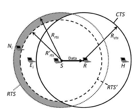
Based on the strategy mentioned in Section Ⅳ-B, the RTS and CTS transmission ranges should be asymmetric. Fig. 3 shows the concept of our proposed method. First we assumed an environment where every node can communicate with its adjacent nodes with a certain transmission rate. In other words, any one node and its adjacent nodes are located within the range of a certain transmission rate. We also assume that RTS is sent at that certain transmission rate or lower and there are some exposed nodes, as in Fig. 3. We name our proposed method Asymmetric Range by Multi-Rate Control (ARMRC) as explained below.
If the range of RTS becomes shorter as the RTS transmission rate becomes higher, some of those exposed nodes begin to fall outside the RTS range and they do not need to hold their transmissions. If the RTS range is completely included in the CTS range, all of them are no longer exposed nodes. Regarding ACK, it only needs to be received by the sender node, so it should be sent at the maximum data rate. Here, we define the Sender Node as
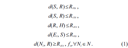
We define the radius of the RTS transmission range by the proposed method, which we configure, as
If formula (2) is satisfied, no Exposed Nodes exist. Also the condition that a node
If formula (2) is not satisfied, Ni satisfying (3) is an Exposed Node. We can define the Exposed Node
Now we can briefly estimate the effect of Exposed Node reduction by ARMRC. With the standard method, any nodes included in
The shaded area of Fig. 3 contains the eliminated exposed nodes by ARMRC and this corresponds to the numerator of formula (5). The total area of both
We show the behaviors described above for ARMRC as follows.
STEP 1: The sender node sends RTS to the receiver node with the highest possible transmission rate. This is to minimize the RTS coverage area and reduce exposed nodes. This means that the number of Ei can be reduced.STEP 2: The receiver node receives the RTS and sends back CTS with the lowest or basic transmission rate. This is to ensure all potential hidden nodes receive CTS and suspend their transmission.STEP 3: The sender node receives the CTS and sends data frame to the receive node with the maximum transmission rate. Some nodes around the sender receive both the RTS and the CTS. Some nodes receive the RTS only, and these are the exposed node. If the RTS range is completely included in the CTS range, there are no exposed nodes. This case corresponds to (2).STEP 4: The receiver node receives the data frame and sends back ACK with the highest transmission rate.
In this section the computer simulation is explained and the proposed method is evaluated.
We assumed the WLAN standard of the 5 GHz band, IEEE 802.11a for our simulation. The system parameters of our simulation are shown in Table 2.
[Table 2.] System parameters for the simulation (ARMRC)
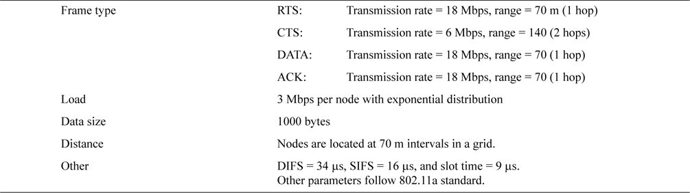
System parameters for the simulation (ARMRC)
In IEEE 802.11a, the eight transmission rates are 6, 9, 12, 18, 24, 36, 48, and 54 Mbps. As we mentioned in Section IV, the transmission rates of RTS and CTS are configured to be asymmetric. In this simulation, RTS is sent at 18 Mbps and CTS is sent at the minimum basic rate of 6 Mbps. DATA and ACK are sent at the same rate as RTS, i.e., 18 Mbps. We used 18 Mbps for RTS transmission rate to show the effectiveness of the proposed method ARMRC. If we used 54 Mbps, the sender and receiver nodes must be located very close to each other compared to the range of RTS/CTS with the basic transmission rate, and this would cause a relatively small number of exposed node. Other data rates could be configured, and these variations will be the subject of our future research as well as theoretical analysis.
2) Network Topology and Traffic Pattern
In this simulation, as an ad-hoc network topology all nodes are located in a grid with 70 m intervals. Seven cases are assumed with grid sizes of 3 × 3 with 9 nodes, 4 × 4 with 16 nodes, 5 ×5 with 25 nodes, 6 × 6 with 36 nodes, 8 × 8 with 64 nodes, 11 × 11 with 121 nodes, and 15 × 15 with 255 nodes. Nodes can be randomly distributed, but in practical deployment distribution of nodes is often governed by artificial objects, such as walls, furniture, partitions, and the structure of building, and as such follow a geometric arrangement. Many structures or objects in our daily life tend to be in a grid arrangement. Roads and buildings in well-developed areas are good examples of this. Another rationale of the grid layout is that we consulted a couple of deployment guidelines from outdoor Wi-Fi mesh vendors [14, 15] and found that those guidelines often start with a grid topology as a grid that is easy to design and often fits well to real world environments. Thereby we assumed a grid distribution for our research. We will definitely exploit other topologies (e.g., random distribution) and mobility of nodes in our future research.
These RTS and CTS distances are based on the ‘distance in this paper’ category in Table 1. Table 1 is compiled based on data in [16, 17] and the free space path loss,
where λ is wavelength and
We assumed the following traffic pattern to simulate various data communication in an ad-hoc network. Each node generates 3 Mbps throughput traffic on average with exponentially distributed data frames, and the destination of each data frame is selected at random from four nodes with a one hop distance. We conducted some trial simulations and found out that 3 Mbps is enough to maximize the entire throughput but not saturate the network. Nodes at the boundary of the network do not have four adjacent nodes and select their destination from fewer candidate nodes at random. In practical deployment adhoc networks may not consist of a large number of nodes and a substantial portion of the nodes can be located on the network boundary. We evaluated the effect of a boundary in our simulation. The simulation continued for five seconds.
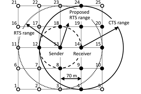
The 5 × 5 grid of 25 nodes is shown in Fig. 4. In this figure node 13 is the sender and the receiver is selected from nodes 8, 12, 14, and 18 at random. In Fig. 4, node 14 is selected as the receiver. An RTS with the standard method reaches up to a node at a two-hop distance and a total of 12 nodes excluding the sender node are in the transmission range. An RTS with the proposed method ARMRC reaches only the nodes at a one-hop distance and a total of four nodes are in the transmission range. As the CTS transmission range has a two-hop distance, the RTS range of the proposed method is completely included in the CTS range and there are no Exposed Nodes. This is the case in formula (2). In this case =
In Fig. 4, black nodes are in the CTS transmission range and white nodes have no influence on the transmission from node 13 to node 14. Gray nodes would be Exposed Nodes if the standard method is applied. These are no longer Exposed Node with the proposed method. This is the case of formula (3).
1) Throughput Comparison with Network Size
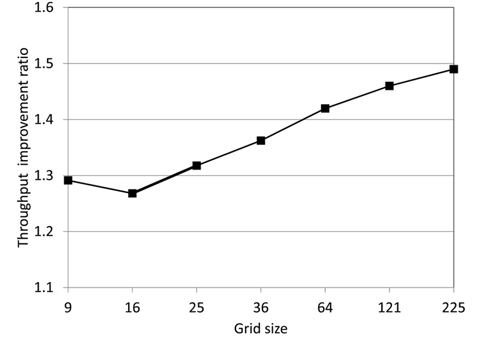
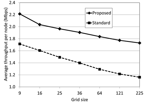
In Table 3, average throughput of a node is shown for grid from 3 × 3 with 9 nodes to 15 × 15 with 255 nodes. Fig. 5 shows a graph of the throughput improvement ratio between the standard method and the proposed method. Fig. 6 is the graph of these average throughputs. All these results were obtained with 3 Mbps traffic generation at each node.
As shown in Fig. 5, for all sizes of grid, the proposed method has improved throughput and the improvement ratio is 27% to 49%. As shown in Fig. 6, throughput pernode descends as the size of the grid ascends for both the standard and the proposed method. However, the entire network throughput increases. Compared to the standard method, the proposed method always has higher throughput and the reason is the reduction of Exposed Nodes.
[Table 3.] Average throughput per node by grid size
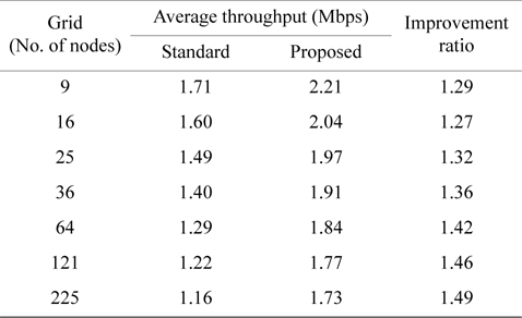
Average throughput per node by grid size
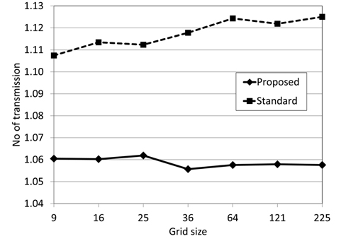
Next we evaluated the effect of RTS collision. The RTS frame is smaller than the data frame and has a lower possibility of causing a collision. When RTS is received safely the NAV's in RTS and the following CTS guarantee the successful transmission of the data frame by suppressing transmission of other nodes around the receiver node [12].
Fig. 7 shows the average number of RTS transmissions per data frame for each grid size. If the number is greater than 1.0, it implies the occurrence of RTS retransmission. Originally RTS/CTS were introduced to mitigate the hidden node problem, but they are also known to have reduced collisions in highly loaded networks [12]. With the standard method, 11% to 13% of RTS were retransmitted due to collisions, and the retransmission ratio becomes higher as the size of the grid becomes bigger. With the proposed method, the average retransmission ratio is lower at 5% to 6%. This does not change when the size of the grid changes. The proposed method can reduce RTS collisions compared to the standard method, and increases throughput.
2) Comparison of Throughput of each node within a Network
Throughput of each node in a network is evaluated in this section. Table 4 shows the improvement ratio in order of improvement. In this table, the network is a 15 × 15 grid with 255 nodes and the improvement ratios of all nodes are sorted in descending order and grouped by every 15 nodes into 15 groups. Both the standard and the proposed method are compiled into Table 4 and each group shows its average throughput for 15 nodes.
[Table 4.] Throughput of a 15 × 15 grid with 255 nodes
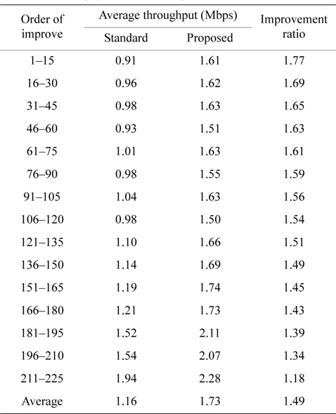
Throughput of a 15 × 15 grid with 255 nodes
As shown in Table 4, we can see substantial variations among the throughputs of all groups. We found that the group which has the highest improvement ratio (1.77) also has the lowest throughput (0.91 Mbps) with the standard method, and the group which has the lowest improvement ratio (1.18) has the highest throughput (1.94 Mbps) with the standard method. This tendency is seen for all sizes of grids, and the proposed method has a stronger improvement effect on lower throughput nodes. The 4 × 4 grid with 16 nodes network in Table 5 has the same tendency.
[Table 5.] Throughput of a 4 × 4 grid with 16 nodes
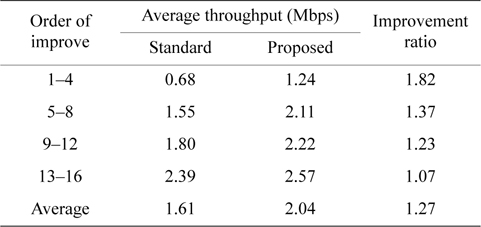
Throughput of a 4 × 4 grid with 16 nodes
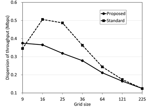
Fig. 8 shows the graph of average throughput dispersion. The proposed method has smaller dispersion than the standard method, and this tendency is more ostensible for smaller grid sizes. We have confirmed that the proposed method levels variation of throughput. For the 15 × 15 grid with 225 nodes there are no differences in dispersion between the standard and the proposed method. We see a tendency that dispersion is converged to a single value as the network size becomes bigger. To the best of our knowledge and experience, there are some commercial ad-hoc network deployments and the size of those deployed networks is small. It is usual to have fewer than 10 nodes, and we would say it is rare to have 100 nodes or more. Therefore this characteristic can be important.
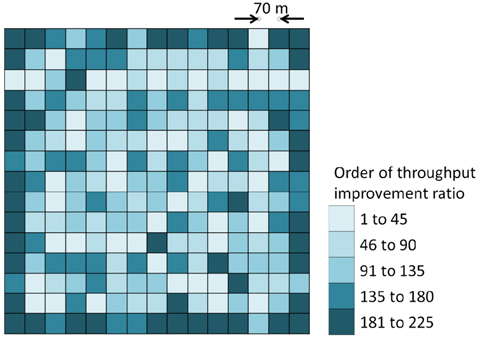
Next we consider effect of the network boundary. As shown in Fig. 4, we anticipate the effect of the boundary to strongly influence the throughput when the size of the grid is smaller than 36 nodes. The effect is expected to decrease as the size of the grid increases. Fig. 9 shows the throughput distribution of the 15 × 15 gird with 225 nodes. As we explained in Table 4, these 225 nodes are divided into 15 groups in descending order of throughput improvement ratio. In Fig. 9, these 15 groups are consolidated into five groups and these five groups have colors based on their throughput improvement ratio. The darker color has a lower improvement ratio and each color represents 45 nodes. The colors stand for relative improvement ratio and not absolute throughput values. There is a strong correlation that high throughput nodes with the standard method attain a low improvement ratio with the proposed method. Still their absolute throughput is high enough even after their improvement. Therefore we can recognize that the dark nodes have a high absolute throughput with both the standard and proposed method. In Fig. 9, high throughput nodes are located at the boundary boundary of the network. These nodes acquire the lowest throughput improvement ratio with the proposed method but still have the highest throughput values. This boundary effect diminishes drastically when the location of a node moves inwards in the grid by just one hop.
3) Evaluation of CTS/ACK Collisions and NAV/CCA
Our proposed method cannot protect CTS and ACK frames completely from being received by the sender node. Consequently, CTS and ACK frames may be lost to collisions caused by nodes around the sender as these nodes are no longer exposed nodes (they do not receive RTS and do not suspend their transmission anymore), then the entire four-way handshaking may fail. However, CTS and ACK are small frames compared to the data frame and we assume that the possibility to lose them by collision is negligible.
Also, as we mentioned in Section Ⅳ-B, our proposed method may still cause exposed nodes due to the PLCP preamble and header. We also assumed this possibility is negligible. If this happens, the exposed nodes should wait for the DIFS plus a random backoff period.
To clarify these considerations, we conducted a supplemental simulation. In Table 6 we show the simulation parameters and in Table 7 we show the result.
[Table 6.] System parameters for the supplemental simulation (ARMRC)
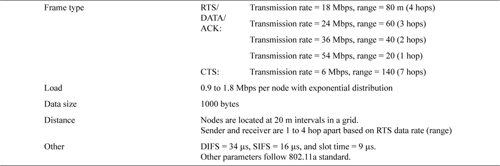
System parameters for the supplemental simulation (ARMRC)
[Table 7.] Result of the supplemental simulation

Result of the supplemental simulation
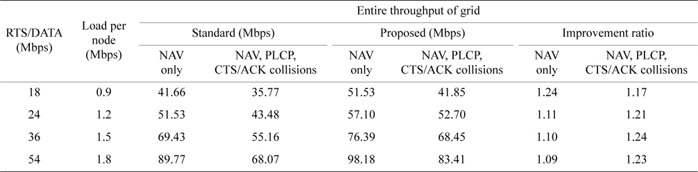
In this simulation we assumed a 15 × 15 grid with 20 m intervals, CTS/ACK (6 Mbps) = 7 hops/140 m and DATA=1 hop/20 m. As in Table 6, the RTS/DATA range is variable and is quantized by units of 20 m, with 4 hops/ 80 m at 18 Mbps, 3 hops/60 m at 24 Mbps, 2 hops/40 m at 36 Mbps, and 1 hop/20 m at 54 Mbps. Thus all RTS ranges except when RTS = 18 Mbps are completely included in the CTS range and there are no Exposed Nodes in order to maximize the effect of the proposed method. In Fig. 10, the grid of RTS/DATA/ACK = 18 Mbps is shown with the same notation as Fig. 4. In this figure big shaded nodes are exposed nodes and this is the only grid which has exposed nodes in this simulation. For other transmission rates higher than 18 Mbps, RTS range is completely included in the CTS range.
In Table 7, ‘NAV only’ means transmission suspension by only RTS/CTS NAV is evaluated. ‘NAV, PLCP, RTS/ ACK collisions’ means in addition to NAV only, transmission suspension by CCA is induced with PLCP and CTS/ACK collisions are also evaluated. PLCP induced transmission suppression and CTS/ACK collisions degrade throughput by 15% to 25% for both the standard and proposed methods. However, the proposed method still shows a 17% to 23% improvement. Hence we can conclude that the transmission range of the PLCP preamble/header and no protection for CTS/ACK do not spoil the gains of the proposed method.
We confirmed that the proposed method has a certain effect by this simulation. By eliminating exposed nodes, it may be possible to improve the entire network throughput by 30% to 50%. It has a stronger effect on low throughput nodes. In the case of small size networks, due to the influence of the network boundary, the effect of our method can be impaired somewhat. However, in our simulation we got a 30% improvement even for a small size network, and also the leveling effect of throughput dispersion is stronger for smaller size networks.
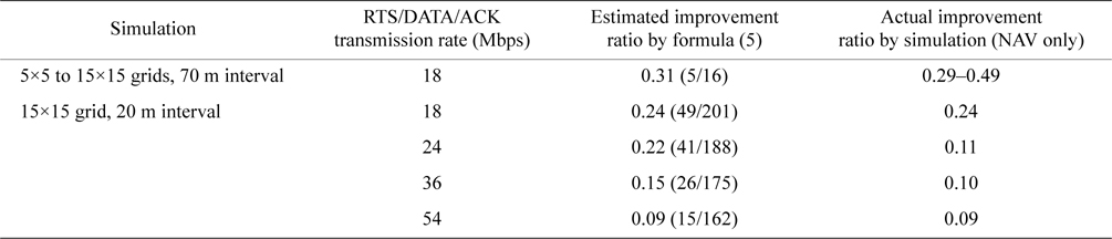
We showed that the throughput improvement ratio could be estimated roughly with formula (5). In Table 8, we summarize the estimated and simulated throughput improvement ratio for comparison.
[Table 8.] Comparison of the estimated and simulated throughput improvement ratio

Comparison of the estimated and simulated throughput improvement ratio
Even though formula (5) is very simple and does not consider any factors other than the number of nodes, it seems to work well. Due to the limitations of simulated finite grid sizes, for most simulated traffic all possible interfering nodes of the sender and the receiver are not in the simulated area. For example, as we see in Fig. 10, all exposed nodes are not in the grid and their influences are not evaluated. We estimate that these deviated or incomplete patterns would cancel each other out and the remaining sum would be close to that for an infinite size of gird. Further theoretical analysis will be the subject of our research from now on.
As multi rate transmission of WLAN expands, difference in the transmission rate between the data and control frames becomes bigger. It can be up to nine times bigger using IEEE 802.11a as the maximum and minimum transmission rates are 54 and 6 Mbps, respectively, and 54 times bigger using IEEE 802.11g with maximum and minimum rates of 54 and 1 Mbps, respectively. As a result there is a substantial difference in transmission range between data and control frames. Hidden node and Exposed Node are problems caused by the spatial distribution of equipment (nodes). RTS/CTS as the resolution mechanism assumes both data and control frames have the same transmission rate, but this is not optimal for a multi-rate environment. In this paper we proposed a new method ARMRC such that by adjusting the transmission rates of RTS to the same as the data frame controls its transmission range proactively. Through simulation we confirmed and quantified the effect of the proposed method. We showed that the proposed method can improve throughput per node by 30% to 50% under certain conditions. Supplemental simulation with CTS/ACK collisions and CCA by PLCP showed around a 20% improvement under certain conditions. With ARMRC we assumed that the RTS transmission rate is the same as the DATA rate and this rate is already known. Using a more general assumption, we say nodes are located with arbitrary distances and we need to define a procedure to find the optimized RTS transmission rate. In future work, we need to investigate further to validate the effect of the asymmetric transmission rate strategy and find a method of selecting appropriate parameters for each network as well as formulating a theoretical explanation for the process involved.