A postulated loss of coolant accident (LOCA) is one of the design basis events that can occur in the primary system of a pressurized water reactor (PWR). The prediction of peak clad temperature (PCT) for the nuclear fuel rod is very important to determine the safety margins during the reflood phase of the LOCA. The behavior of the entrained droplets generated at the quench front of reflooding water crucially affects the reflood heat transfer by decreasing the superheated steam temperature and interacting with the rod bundle and spacer grids (Ergun, 2006).

Spacer grids are an intricate part of the fuel assembly design, whose role is to provide support for the fuel rods and maintain a constant distance between rods in a tight lattice, secure flow passage, and prevent damage to the assemblies from flow-induced vibration. A noticeable enhancement of the heat transfer from the rod bundle was observed due to the presence of droplets and their interaction with the grid spacer, especially in the dispersed flow film boiling regime (Cheung and Bajorek, 2011). The droplets, which are characterized by large surface area-to-volume ratios, provide a significant amount of interfacial area for heat and mass transfer. Evaporation of the droplets downstream causes the vapor temperature to decrease and the vapor flow rate to increase. Both would lead to a higher rate of cooling of the rods, thus lowering the PCT. Because the droplet behavior and interfacial area for the heat and mass transfer between the droplets and superheated vapor can significantly change as the twophase mixture travels through a grid spacer, the interaction between grid spacers and droplets should be taken into account and modeled in the safety analysis for the prediction of peak clad temperature of a nuclear fuel rod.

The effects of a dry grid spacer on the droplet size and distribution have been experimentally investigated by Lee et al. (1984), Sugimoto and Murao (1984), and Ireland et al. (2003). Cheung and Bajorek (2011) theoretically studied the dynamics of droplet breakup associated with the flow of a dispersed two-phase mixture through a dry grid spacer. By considering the conservation of liquid mass, and the kinetic and the surface energies of the droplets, they derived an expression for the ratio of the Sauter mean diameters of the droplets downstream and upstream of the grid, which was compared well with available data.

The RBHT test facility was constructed to investigate the flow and heat transfer characteristics within the bundle assembly for the case of an LOCA, where a series of droplet injection experiments have been carried out to investigate the grid effects on the rod bundle heat transfer (Srinivasan, 2010). The results of this experiment showed that those grids in the upper portion of the rod bundle could become wet well before the arrival of the quench front even under low-flooding-rate conditions and moreover that the sizes of liquid droplets downstream of a wet grid were considerably larger than those produced by a dry grid, indicating a distinctly different droplet formation mechanism. For a wet grid spacer, a thin liquid film is present which can be sheared off by the steam flow to form liquid ligaments and large droplets downstream. The wet grid phenomenon can be postulated to consist of four individual processes (Srinivasan, 2010). The first process involves the deposition of droplets from the dispersed two phase mixture onto the spacer grid surface, the second involves the establishment of a liquid film of equilibrium thickness on the surface of the spacer strap, the third involves the entrainment of liquid ligaments from the liquid sheet due to the shear action of the steam flow, and finally, the fourth involves the breakup of these ligaments into a number of fine droplets downstream of the grid.

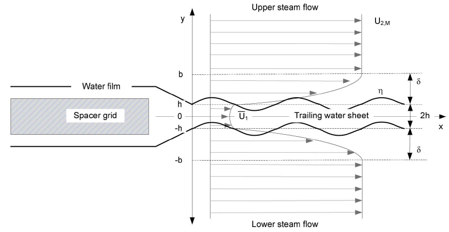
This study is aimed at developing a theoretical model for water droplet generation from a wet grid spacer and examining the effect of physical parameters on the downstream droplet diameters. Special attention is given to the instability mechanism at the water/steam interface as a thin water sheet issues from the trailing edge of a wet spacer grid with a surrounding steam up-flow. To this end, a sophisticated mathematical formulation which has recently been developed in atomization and spray research is adapted, where shear and normal stresses at the interface are conserved in the steam and liquid basic flows, as well as in their perturbations. In this formulation, the interfacial boundary conditions correctly reflect the actual flow situation, including pressure and viscous stresses in balance with surface tension forces. Velocity profiles at a given downstream location are approximated by parabolic ones satisfying the velocity and shear stress continuities. The Orr–Sommerfeld differential equations and boundary conditions of the flow configuration are numerically solved using Chebyshev series expansions and the Tau–Galerkin projection method.

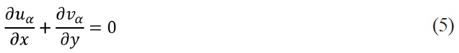
Cho (2011) investigated droplet behavior inside a 6×6 rod array for the droplet break-up phenomena caused by a wet grid spacer and during the reflood phase of an LBLOCA. His results showed that the shattering of droplets into a number of small droplets was clearly observed for the case of a dry grid spacer. For the tests with a wet grid spacer, however, a liquid film covered the mixing vane and grid spacer, and droplets were generated from the tearing of the liquid sheet off the end of the mixing vane with a hydrodynamic break-up process. The shear action of the steam flow induces a velocity in the liquid film which then issues from the trailing edge of the spacer grid as a viscous water sheet. The water sheet is subsequently disintegrated into several droplets due to aerodynamic and capillary instabilities. While there was no apparent correlation between the ratios of droplet Sauter mean diameters upstream and downstream of the grid spacer and the steam velocity, the Sauter mean diameter itself at the grid spacer downstream and the steam velocity had a fairly good correlation. Since all the incoming droplets were de-entrained on the grid spacer and form a liquid film in the experiment, the size of the droplets upstream of the grid spacer did not have any significant influence on the resulting droplet size change across the grid spacer.

The droplet entrainment rate from a liquid film has been an important research subject in analyzing heat and mass transfer processes in an annular two-phase flow, where mass, momentum, and energy transfer processes are strongly affected by the amount of droplets in the streaming gas. Theoretically the amount of droplet entrainment can be determined by the integral balance between the droplet entrainment rate and the droplet deposition rate. Based on the mechanistic model of shearing off of roll-waves by the streaming gas, correlations for the inception of droplet entrainment, the amount of entrained droplets for a steady state flow, and the distribution of droplet size has been developed (Kataoka et al., 2000). Most correlations and experimental data for both droplet deposition and entrainment, however, have been developed for annular flow in a duct of a circular cross section or flat plates, neither of which are similar to the flow cross section of a rod bundle with a spacer grid. In addition, the film thickness on the surface of a wet spacer grid is expected to be very small, so the entrainment from a wet grid is not expected to be identical to the conventional annular flow entrainment mechanisms, namely, shearing off of the roll wave crests or wave undercutting.

Spray and atomization have been important research subjects for many practical applications. The destabilization and breakup of liquid streams have been studied extensively for more than a century for the efficient design and operation of sprays. For air-assisted configurations, the air stream flows at a much higher speed surrounding the liquid. The aerodynamic forces acting on the surface of a liquid sheet cause waves to be generated on its surface. Fragmentation of the sheet occurs due to the growth of these waves. Once the amplitude of these waves reaches a critical value, liquid ligaments are torn off from the sheet, deforming into cylindrical ligaments. Capillary forces then cause these ligaments to further break up into spherical droplets.

The linear instability analysis of the liquid sheet problem was initiated in the works of Squire (1953) and York et al (1953). In these two studies, water was considered to be inviscid, moving in a quiescent ambient air. Hagerty and Shea (1955) repeated a similar study, comparing the predictions with their own experimental measurements. They found that in liquid sheets, unlike round jets, surface tension has a stabilizing effect; thus, capillary instability does not exist for this type of flow. They also concluded that sinuous mode was generally more unstable than varicose mode.

Dombrowski and Johns (1963) studied the aerodynamic instability and disintegration of viscous sheets in a quiescent inviscid gas. They found that under some flow conditions, the sinusoidal mode dominates and grows faster than the varicose mode. Li and Tankin (1991) carried out a temporal instability analysis of a moving thin viscous liquid sheet in an inviscid gas medium. Their results showed that surface tension consistently opposed, while surrounding gas and relative velocity between the sheet and gas favored, the onset and development of instability. It was also found that there existed two modes of instability for viscous liquid sheets, i.e., aerodynamic and viscosity enhanced instabilities.

Teng et al., (1997) investigated the linear instability of a viscous liquid in a vertical sheet sandwiched between two viscous gases bounded externally by two vertical walls using spectral methods with Chebyshev series expansion to solve the Orr–Sommerfeld equation. It was found that the sinuous mode had a greater amplification rate than the varicose mode in the convective instability regime. While absolute instability was caused by the surface tension, convective instability was caused by the amplification of disturbances near the liquid-gas interface. Ibrahim et al., (1998) analyzed the linear stability of an inviscid liquid sheet emanated into an inviscid gas medium. The influences of Weber number and the gas/liquid density ratio on the evolution of two and three dimensional disturbances of symmetrical and anti-symmetrical types were studied. Barreras et al. (2001) studied the evolution of sinusoidal waves propagating on a water sheet surrounded by two high-velocity co-flowing air streams. Their analysis was based on linear instability theory and included viscosity in both gas and liquid perturbations, while for the stationary velocity profiles the flows were treated as inviscid.

Hauke et al, (2001) applied the temporal linear instability analysis to a thin planar liquid sheet flowing between two semi-infinite streams of a high-speed viscous gas. Their study included full viscous effects both in the basic states and perturbations for the liquid and gas. The Orr–Sommerfeld equations and boundary conditions were formulated and numerically integrated. Only the sinuous mode was investigated on the basis of experimental observation. They concluded that the momentum flux ratio was especially relevant to determine the instability conditions, and that the gas boundary layer thickness strongly influenced the neutral stability curve.

Altimira et al., (2010) recently derived the Orr–Sommerfeld differential equations from fundamental governing equations for a viscous two-dimensional liquid sheet and numerically solved these equations and boundary conditions using Chebyshev series expansions and the collocation method. The dependence of the instability parameters on the velocity profiles was studied by using quadratic and error functions to define the base flow in the liquid sheet and the gas shear layer. The steep gradients of gas shear flows required a spatial discretization with clustering of the elements near the boundaries. Even though he adopted a set of collocation points from the Gauss–Lobatto grid method, a strong sensitivity of the solution to the value of the clustering parameter was observed.

Cho’s visual experiment (2011) for the wet spacer grid clearly showed that the mixing vane and the grid were covered by a liquid film, and droplets were then generated from the tearing of the liquid sheet off the end of the mixing vane. The droplet generation process through the wet grid can be divided into the following four steps:

(1) Liquid droplets contacting the grid form a water film on it.

(2) A water sheet issues from the trailing edge of a wet spacer grid.

(3) The water sheet is broken up into ligaments due to an interaction with the surrounding steam flow.

(4) Each ligament is further disintegrated into droplets due to capillary force.

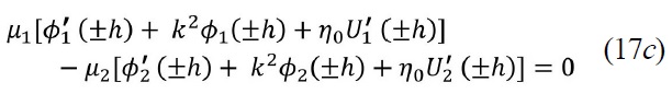
The fraction of incoming droplets that will form the water film on the surface of the spacer grid is expected to be a function of the blockage ratio of the grid spacer. The fraction of droplets contacting the spacer grid along the flow path inside the fuel assembly is proportional to the blockage ratio. Assuming all the droplets contacting the grid form a water film on the grid space, the fraction of incoming droplets forming the film is equal to the blockage ratio and the remaining fraction escapes through the spacer grid. The water film is transformed into a water sheet just downstream of the grid and the sheet thickness will gradually decrease by acceleration. As the instability just begins to develop downstream of the grid, the trailing thickness of the sheet is approximately twice that of the water film. The water sheet is broken up into several ligaments due to a dynamic interaction with the surrounding steam flow, and each ligament is then further disintegrated into spherical droplets due to capillary force.

A linear perturbation analysis is based on perturbing a steady-state solution of a flow with a small-amplitude wave in the normal mode, analyzing its growth rate with the linearized Navier-Stokes equations. The wave amplitude has to be small compared with its wavelength and with the sheet thickness for validity of the linear perturbation analysis.

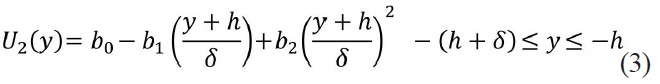
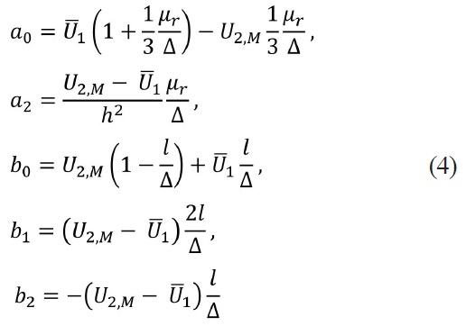
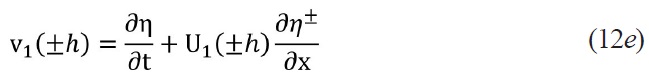
Consider a thin water sheet sheared by a steam flow downstream of the trailing edge of a spacer grid as sketched in Figure 1. The linear stability analysis model for a twodimensional sheet of constant thickness, 2h, of viscous water sandwiched between two identical viscous steam streams is developed. Steam flows are characterized by the median velocity U_2,M and by the boundary layer thicknesses, δ. The median velocity, U_2,M refers to the velocity at the center line in the absence of a spacer grid. The steam velocity profile is very uniform near the center of channel and the disturbed portion by the existence of the spacer grid is limited to its close proximity, so the deformation of basic steam flow is assumed to be limited to inside the boundary layer. The upper and lower steam flows interact with the liquid sheet through pressure and viscous stresses at the interfaces y = ±h. Water and steam phases are identified by subscripts 1 and 2, respectively. The basic velocity profiles for the water sheet and the steam boundary layer were approximated by a quadratic function of y, independent of the downstream coordinate. The unperturbed velocity profiles were approximated by

where h ≤ y ≤ h+δ for the upper steam flow and –(h+δ) ≤ y ≤ –h for the lower steam flow. The unknown coefficients a_i and b_i were calculated by imposing the following constraints (Hauke et al, 2001).

- The water mean velocity,

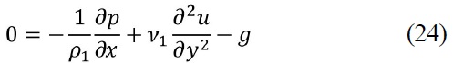
is given.

- The steam and water velocities at the unperturbed interfaces, y = ±h, are equal.

- The tangential viscous stresses balance at the unperturbed interface.

- The steam median velocity in the fuel channel, U2,M is given.

- The steam velocities at the boundary layer edges, y = ±(h + δ), are equal to U2,M.

- The steam velocity gradients at the boundary layer edges vanish.

We can obtain five algebraic equations after applying the above constraints. Solving the equations yields

where μ_r = μ₂/μ₁ is the steam/water viscosity ratio, l = δ/h is the ratio of the steam boundary layer thickness to the water sheet half thickness, and Δ= (2/3)μ_r + l. Usually the mean steam velocity is known for the existing experimental results, instead of the median velocity, U_2,M, used above. The median velocity can be calculated from the mean value if we introduce the 1/7^th power law velocity profile for the turbulent channel flow.

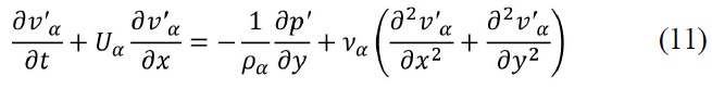
The governing equations for the water sheets and the surrounding steam flow are

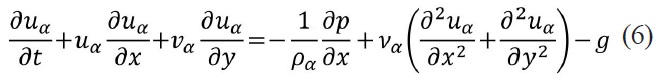
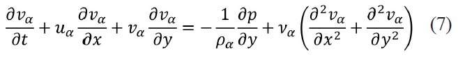
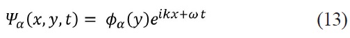
where ρ is the density, ν the kinematic viscosity, and α=1 refers to the water phase, whereas α=2 denotes the surrounding steam. The perturbed flow fields are given by

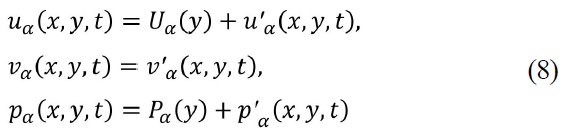
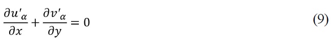
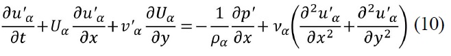
In the above expressions, the magnitudes in capitals represent the values of the corresponding field for the base flow, and magnitudes marked with prime represent the disturbed components of the flow variables. The linearized governing equations of the disturbed flows are

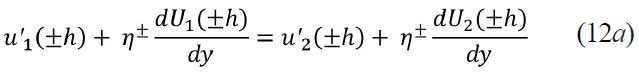
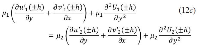
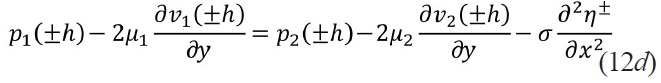
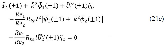
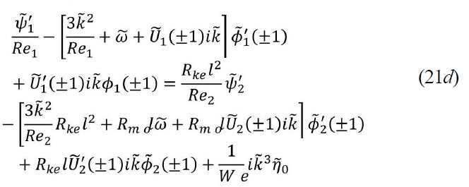
The appropriate boundary conditions are velocity continuity and stress balance across the interface plus the kinematic condition, derived from considering the equation of the interface S(x, y, t) = η^±(x, t) – y = 0, where η⁺ (x, t) and η^–(x, t) are the upper and lower interface displacements from the equilibrium position, respectively. The values of flow variables at the interface y = h + η^± are taken as a firstorder approximation about y = ±h. Hence, the imposed boundary conditions can be described as follows:

Continuity of velocities

Continuity of tangential stress

Jump of normal stress

Kinematic condition

To complete the set of equations, the perturbations must die away at locations far from the interfaces.

This gives

The viscous two-dimensional problem can be conveniently solved in terms of the stream function, Ψ(x, y, t) formulation. The perturbed flow stream functions in normal mode decomposition can be expressed by

where φ_α(y) are the amplitudes of the normal mode disturbances, k is the real wavenumber of the perturbation, and k=2π/λ, where λ is the wavelength of the disturbance, and ω=ω_r+ω_i is a complex frequency. The real part of complex frequency, ω_r, represents the rate of growth or decay of the disturbance while its imaginary part, ω_i, is the disturbance frequency and ω_i/k is the wave propagation velocity of the disturbance. Hence, the disturbance frequency and wave velocity are related. A temporal instability method where disturbances are assumed to grow temporally everywhere is chosen for this study. It has been utilized for several former studies for liquid sheet instability analyses (Li and Tankin, 1991, Hauke et al, 2001, and Rangel and Sirignano, 1988). Gaster (1962) showed that for small rates of amplification, the disturbance frequencies determined from the temporal theory were approximately equal to those of the spatial analysis. The Stokes stream function is related to the x- and y-components of the disturbance velocity by

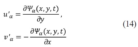
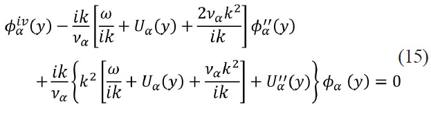
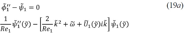
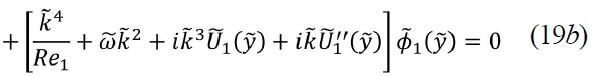
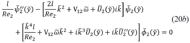
The definition of the above stream function naturally satisfies the continuity equation. If we apply the function to the two momentum equations for the disturbed flows, we can get two coupled Orr-Sommerfeld equations after some manipulation. The linear stability of the basic state with respect to the normal mode two-dimensional perturbations is governed by following two coupled Orr-Sommerfeld equations.

The perturbed thickness of the water sheet can also be expressed in the normal mode decomposition as follows:

By applying the normal mode decompositions for the stream function and sheet thickness to the boundary conditions, the following equations can be obtained.

Continuity of velocities

Continuity of tangential stress

Jump of normal stress

Kinematic condition

The boundary conditions for vanishing perturbation velocity away at the locations far from the interfaces can be expressed in the following way:

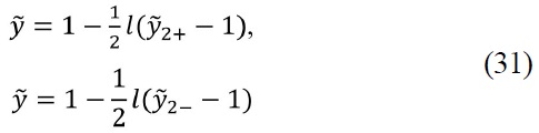
Before proceeding, the variables are transformed into a non-dimensional form, using the appropriate velocity and length scales for both steam and water flows, yielding

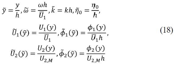
This non-dimensional analysis transforms the water domain into –1 ≤

≤ 1 + l, and the lower steam domain to –(1 + l) ≤

≤ –1, where l = δ/h. In this way, the final Orr-Sommerfeld equations are:

where V12 =

is the velocity ratio.

For the application of the Tau spectral method, the occurrence of spurious eigenvalues has been discussed by several authors (Gardner et al., 1989; McFadden et al, 1990). Gottlieb and Orszag (1977) showed that the spurious roots in the Chebyshev Tau method could be eliminated if the function ψ = φ" was introduced. Dongarra et al., (1996) examined the Chebyshev Tau method in detail for a variety of eigenvalue problems arising in hydrodynamic stability studies. After comparing the method employing a Chebyshev representation of the fourth derivative operator, D⁴, with those involving the second and first derivative operators, D² and D¹, respectively, they recommended the D² alternative because it had better growth properties than the D⁴ one, whereas it made more efficient use of the QZ algorithm than the D¹ method which requires matrices that are twice as large. Following this reasoning, a new function ψ is introduced into Equations (19) and (20) for the removal of a spurious solution and for better convergence. The boundary conditions can also be written in the following non-dimensional forms:

In the above equations Re₁ =

is the water sheet Reynolds number, Re₂ = U_2,Mδ/ν2 is the surrounding steam flow Reynolds number, We =

is the Weber number, R_ke =

is the kinetic energy ratio, and R_mo = ��₂U_2,M

is the momentum ratio. Two final boundary conditions are imposed to the locations far from the interfaces. For numerical analysis with a confined calculation domain, the inviscid solution of the outer steam flow obtained by Hauke et al (2001) is matched with the shear layer flow at

Both conditions at the location far from the interface are replaced by imposing the continuity of steam velocity and normal stress on both sides of the fictitious interface at

Thus, the new boundary conditions are

These boundary conditions allow the investigation of viscous instability in the domain far from the interface, including the steam flow effects and steam boundary layer thickness.

(1) Equilibrium water film thickness

The primary focus of this study is to develop a linear stability analysis model for water sheet breakup due to the shearing action of the surrounding steam flow. A simple balance model will be utilized to calculate the equilibrium thickness of the water film on the grid spacer (Srinivasan, 2010). This equilibrium thickness value can be obtained through a combined mass, force, and energy balance on the liquid film by invoking suitable simplifying assumptions. Since the thickness of the water film is expected to be much smaller than the dimensions of the spacer grid structure, the inertia of the flow in the film can be ignored. In addition, the velocity of the water film can be approximated to be invariant in the x and z (out of the plane of the film) directions. Accordingly, the Navier Stokes equation governing the flow of the water in the flat film portion of the water film can be written as

The above equation can be integrated twice to yield the velocity of the water film. The integration constants can be determined using the no slip and interfacial shear boundary conditions. Finally the average liquid velocity in the flat film can be determined as:

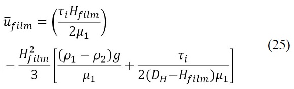
The above equation is the third order equation for the water film, H_film. The H_film can be easily calculated by applying the Newton iteration method to equation (25) for a given water flow rate.

(2) Droplet diameter

The water sheet is separated into several ligaments and their sizes can be obtained on the basis of the specific wave number corresponding to the maximum growth rate. The ligament further disintegrates into individual droplets according to Rayleigh’s theory for the instability of cylindrical liquid columns. The newly generated droplet mean diameter, d_gen, can be obtained from the conservation of mass. The liquid sheet breaks off at half wavelength intervals to form ligaments under the effect of surface tension and aerodynamic interactions (Jazayeri and Li, 1997). The diameter of the resulting cylindrical ligament can be determined from the volume of liquid per unit width in a half wavelength of the sheet as follows:

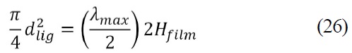
The wavelength λ is equal to 2π/k,

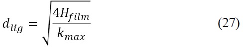
The ligament so produced further disintegrates into individual droplets according to Rayleigh’s theory (Dombrowski and Johns, 1963) for the instability of cylindrical liquid columns. Droplets are formed from a ligament breakup at one wavelength intervals due to the unstable waves on the ligament surface, where the wavelength is given as

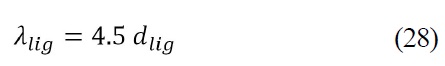
This is the dominant wavelength for the breakup of a cylindrical liquid ligament of diameter, d_lig. Therefore, the resulting droplet mean diameter, d_gen, can be obtained from the conservation of mass as:

The above equations give the final expression for the Sauter mean droplet diameter, d₃₂:

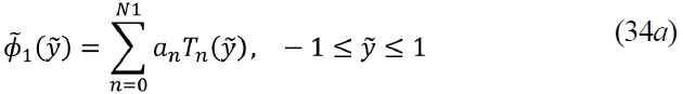
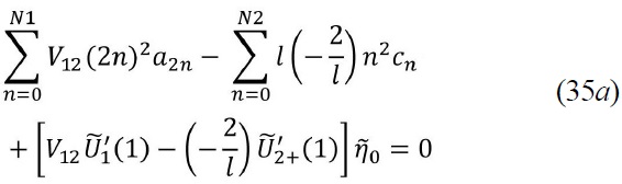
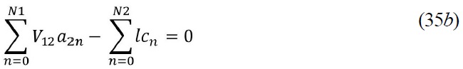
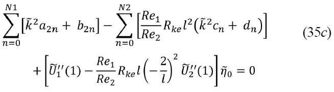
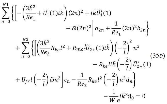
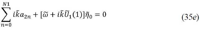
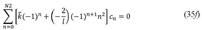
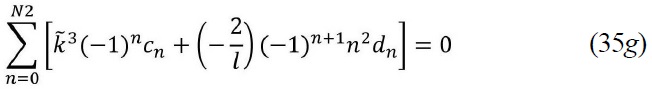
To solve the system of coupled Orr–Sommerfeld equations described in section 3.1, the Tau–Galerkin projection method is employed. The solution space is expanded in Chebyshev polynomials, which are defined in the closed interval [–1, 1]. The procedure is illustrated in detail in the references (Orszag, 1971; Gottlieb and Orszag, 1977; Teng et al., 1997). Since there are two media, the computational domain was divided into three zones: one water domain surrounded by two steam domains. For the uniform steam zones, analytical solutions for the perturbation were derived and then used as boundary conditions for the steam boundary-layer regions. Within each zone the spatial coordinates must be mapped to [–1, 1] in Chebyshev polynomials. The steam domains

and

are mapped into

and

∈ [1,?1] , respectively, by use of the following linear transformations (Teng et al., 1997).

In the new variables,

the expressions of the Orr-Sommerfeld equation and its boundary conditions remain the same except that the n^th derivatives appearing in these equations must be multiplied by (–2/l)ⁿ. The equations for the basic velocity profiles are also nondimensionalized and changed after introducing the change of variables as follows:

The corresponding perturbation amplitude can be expanded in the series of Chebyshev polynomials of n^th degree

Since the governing system of equations is linear and homogeneous, the solution can be separated into even and odd functions of y for the water sheet. The even mode (the symmetric solution, formed by functions with even powers of

i. e. a_2n+1 = 0) generates the sinuous mode. The odd mode (the anti-symmetric solution, formed by odd powers of

i. e. a_2n = 0) generates the varicose mode. For the case of

and

the even and odd powers are not decoupled. The sinuous mode is obtained by retaining the even expansion for

and

while the varicose mode is obtained by retaining the odd terms in the expansion. Attention will focus on the sinuous mode since the sinuous mode has been found to be the dominant instability mode for air-assistant water sheet breakup. Lozano et al. (2009) mentioned in their experimental results for the air-coflowing oscillating sheet that there was no experimental evidence of the presence of varicose waves of measurable amplitude in an air-blasted situation, and only the sinuous ones have been characterized. Rangel and Sirignano (1991) took the sinuous mode as the dominant instability mode for the range of Weber numbers and density ratios explored in the present paper.

The boundary conditions for the sinuous mode, at

= 1 are

The boundary conditions at y₂₊ = –1 are

In the above boundary conditions, the following properties of Chebyshev polynomials are taken into account.

The unknowns are the coefficients of polynomials for the water domain, a_2n, b_2n(0 ≤ n ≤ N₁), those for the steam domain, c_2n, d_2n(0 ≤ n ≤ N₂), and the sheet thickness

There are 2N₁ + 2N₂ + 3 unknowns that should be solved using the above equations. In the Tau–Galerkin method, the boundary conditions are imposed as additional equations which replace the higher order projections. Thus, 0 ≤ n ≤ N₁ –1 equations are retained for the water domain and 0 ≤ n ≤ N₂ –2 for the steam domain; seven boundary conditions are added in order to close the system of equations. The computation of the generalized eigenvalue problem with complex variables was solved with the DGVLCG routine which was included in the IMSL library. DGVLCG is a double precision version of GVLCG. The GVLCG routine is based on the routines developed by Garbow (1978) for the generalized complex eigenvalue problem. The QZ algorithm was described by Moler and Stewart (1973).

The Equations (19a), (19b), (20a), (20b) for dispersion relation were derived from the governing equations for the water sheet and surrounding steam flow, which are solved with boundary conditions employing the Tau-Galerkin method, expanding the solution space in the Chebyshev polynomials. To test the possible syntax and computer program errors, the results for the special cases were checked against the known results of a plane Poiseulle flow (Orszag 1971). Since Orszag had initially solved the Orr-Sommerfeld equation for the Poiseulle flow using expansions in the Chebyshev polynomials and the QR matrix eigenvalue algorithm, several other studies for the spectral method development have benchmarked their methodologies using his result (Gardner et al., 1989; McFadden et al., 1990; Hauke et al., 2001). Orszag found that the critical Reynolds number was 5772.22 for the Poiseulle flow. The critical Reynolds number is defined as the smallest value of Reynolds number for which an unstable eigenmode exists. The numerical scheme developed in this study regenerated the same critical Reynolds number for the instability of a plane Poiseuille flow.

In the temporal stability analysis, a non-dimensional complex temporal frequency value

is obtained for each non-dimensional real wavenumber

Temporal growth occurs for the positive real part

The imaginary part of the temporal frequency

corresponds to the nondimensional wave disturbance frequency. The slope of graph

as a function of

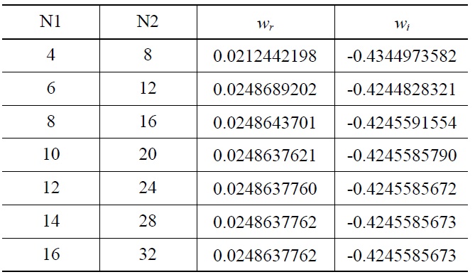
is equal to the relative wave propagation speed to the water velocity. To determine an adequate size of Chebyshev polynomial, sensitivity calculations were carried out. Table 1 shows the typical convergence of the eigenvalue of maximum amplification with increasing N1 and N2 values. These results were obtained for the geometric data and operating condition of the RBHT (Srinivasan, 2010). Table 1 shows that convergence of the eigenvalues can be achieved if N1 and N2 are set to be larger than ten and twenty respectively. The following calculations for sensitivity evaluation will

be performed with N1 and N2 values large enough to guarantee the convergence of the eigenvalues.

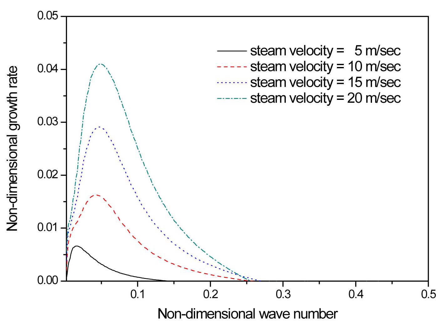
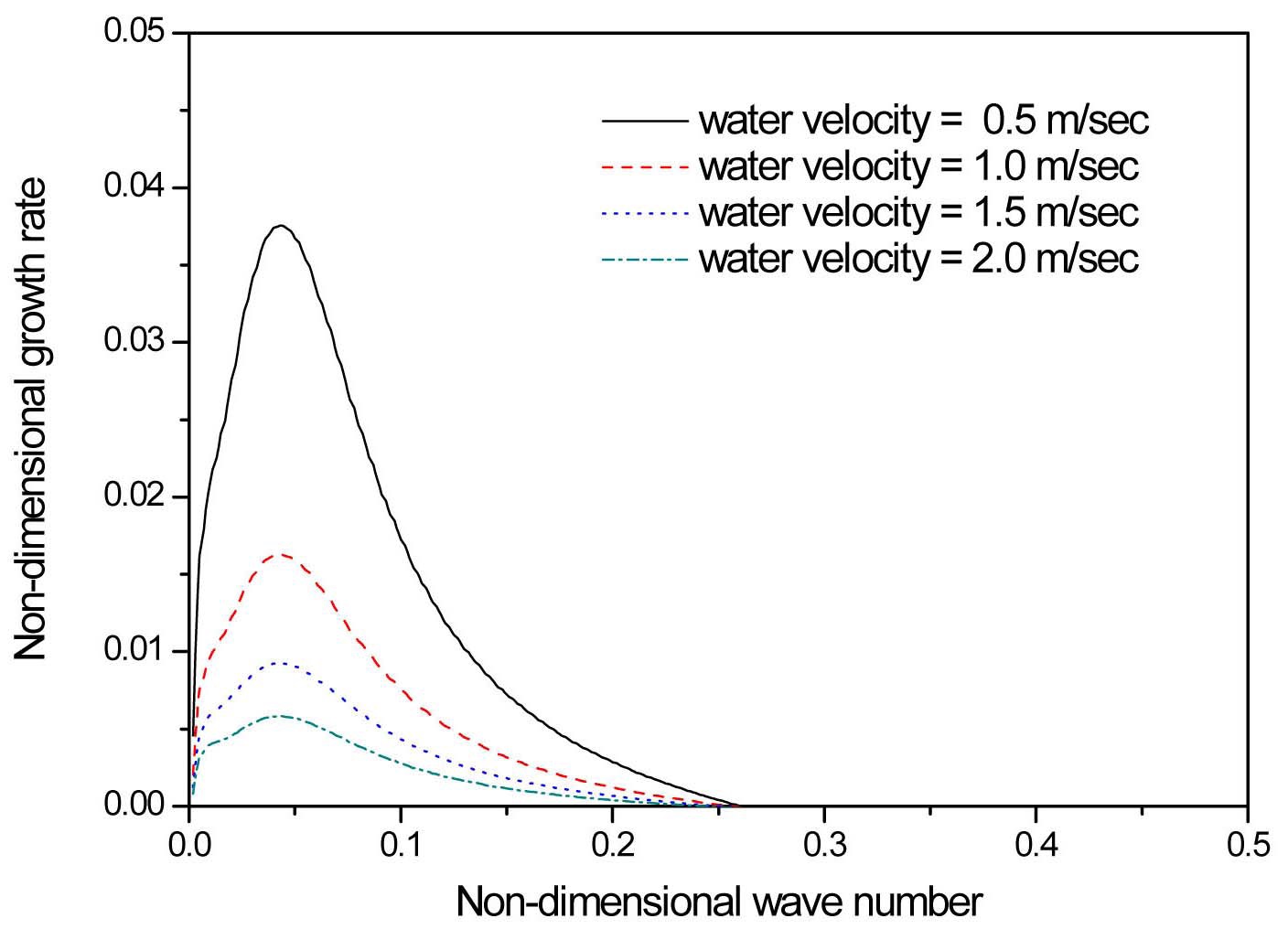
Figures 2 and 3 show the non-dimensionless temporal growth rates as a function of non-dimensional wavenumber for several steam and water velocities, respectively; maintaining all the remaining fluid properties and thicknesses constant. In Figure 2, the steam velocity is varied from 5 m/s to 20 m/s while keeping the water velocity constant at 1m/s. On the other hand, in Figure 3 the steam velocity is fixed at 10m/s and the water velocity is varied from 0.5m/s to 2 m/s. The water sheet velocity is selected on the basis of the practical values for water film on the spacer

grid, which are typically very low due to the large wall frictional resistance. The steam temperature and pressure are 400 ℃ and 0.15 MPa. The water temperature is set to the saturated value corresponding to the steam pressure. It can be observed in the figures that all the curves have a range for which the growth rate is positive, i.e., for which unstable waves can propagate, and all of them present a maximum for a determinate wavenumber, corresponding to the most unstable mode.

As the steam velocity increases in Figure 2, the unstable region broadens, and the maximum growth rates notably increase and are displaced toward larger wave numbers. This result evidently shows the strong destabilizing effect of the steam velocity on the water sheet. The Sauter mean droplet diameters generally have a tendency to decrease as the steam velocity increases in the experiment (Srinivasan, 2010; Cho et al 2011). Contrary to the steam velocity variation, the maximum growth rate decreases as the water velocity increases as shown in Figure 3. Its location slightly shifts toward smaller wave numbers. The increment of water velocity induces the reduction of relative velocity between the steam and water velocities, and resultantly a smaller kinetic energy ratio, R_ke and momentum ratio, R_mo, which has a stabilizing effect on the water sheet. The fact that the wavenumber corresponding to the maximum growth rate is insensitive to the water velocity variation is in good agreement with Cho’s experimental data (2011), which indicate that the dependence of the droplet size on the water flow rate is much weaker than that on the steam flow rate.

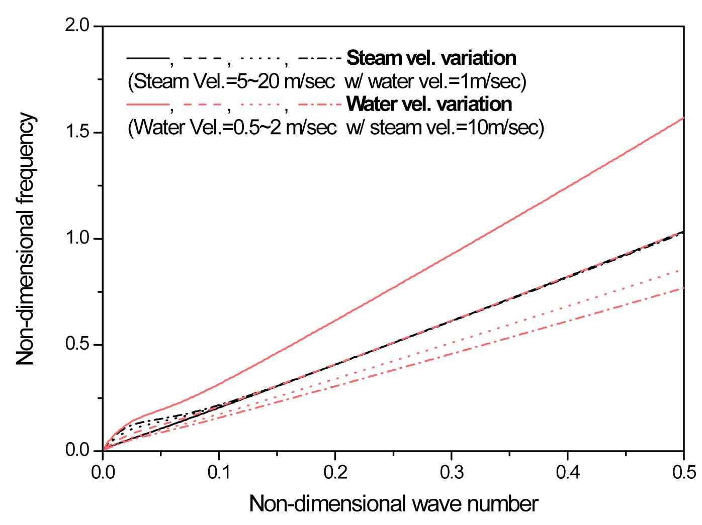
The imaginary part of the temporal frequency as a function of wavenumber is presented in Figure 4. Two cases for the steam and water velocity variations are combined into one graph. The black lines are calculated from the

steam velocity variations, and the grey lines from the water velocity variations. The slope of this curve corresponds to the relative wave propagation speed to the water velocity. Figure 4 shows that the non-dimensional frequency and wave propagation speed are practically insensitive to changes in the steam velocity. The wave propagation speed maintains about twice the water velocity. On the other hand, the wave propagation speed has a decreasing trend as the water velocity increases.

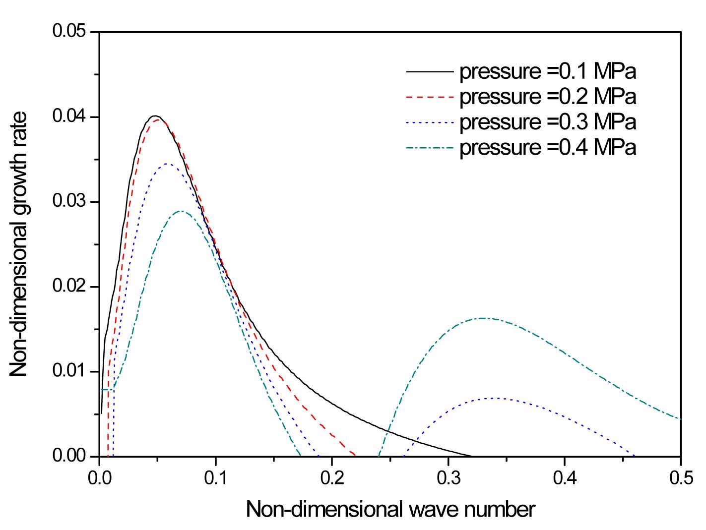
The effects of the operating conditions on the water sheet instability are shown in Figures 5 to 7. In figure 5, the pressure is varied from 0.1 MPa to 0.4 MP while keeping other variables constant. This pressure range was selected to cover the operating conditions of RBHT (Hochreiter et al, 2010). As the system pressure varies, the steam density is mainly affected in such a way that its density increases from 0.32 kg/m³ to 1.29 kg/m³. The variation of steam dynamic viscosity and the water properties are insignificant forure change. The increment of steam density corresponds to a larger steam Re number, Re₂, kinetic energy ratio, R_ke, and momentum ratio, R_mo. The maximum nondimensional temporal growth rates shown in Figure 5 displace toward larger wave numbers, resulting in a shorter wave length and smaller droplet diameter. However, the unstable regions have tendencies to become narrow asures increase. Ifure is larger than 0.3 MPa, the new local peaks emerge at the higher wave number and grow withure increment. The local peaks at a higher waver number are smaller than the original peaks at a lower waver number inure range studied in this study.

Steam is generated from the quench front region during the reflood period and its temperature increases with the heat transfer from the fuel rods as it flows up.

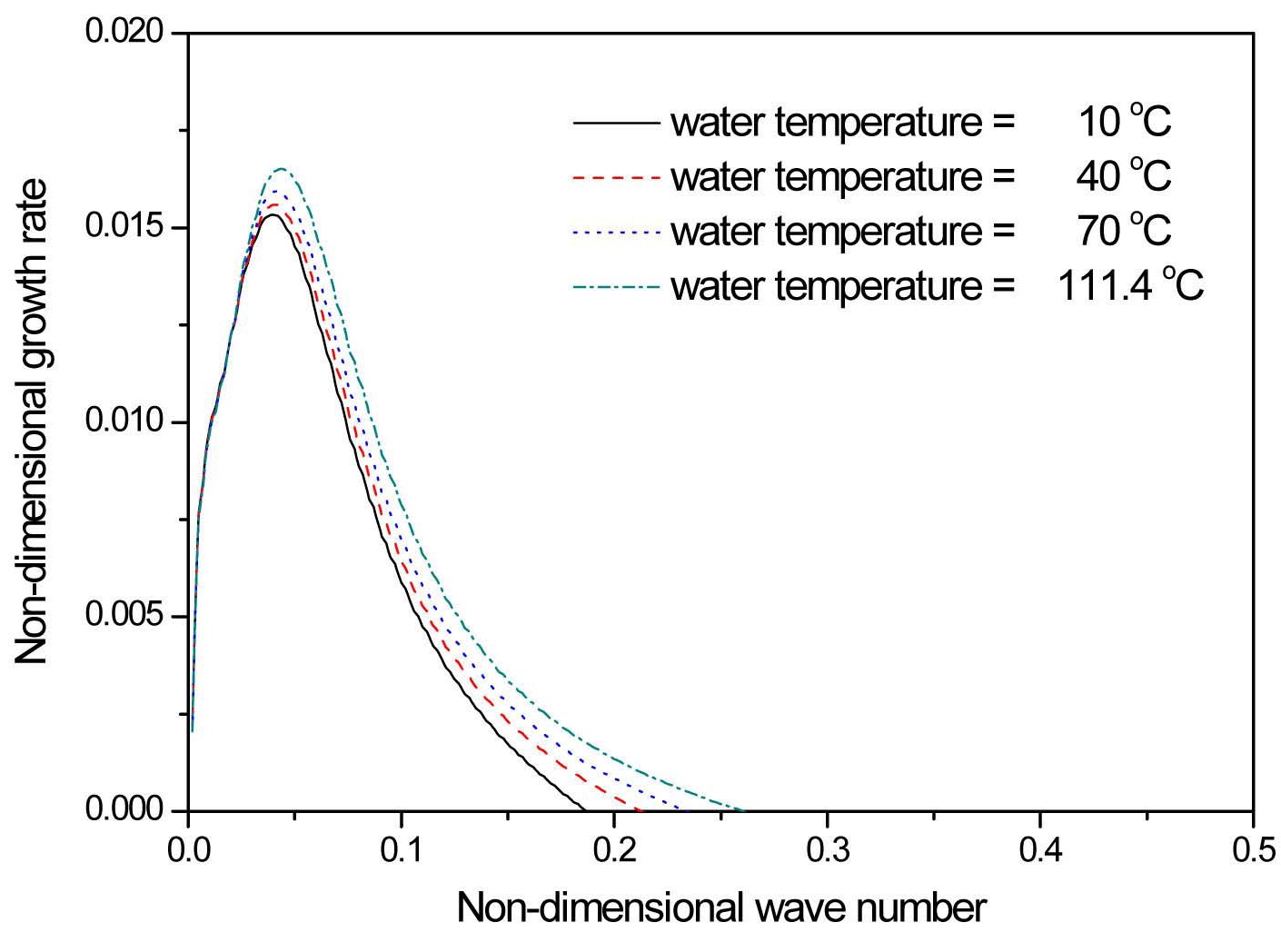
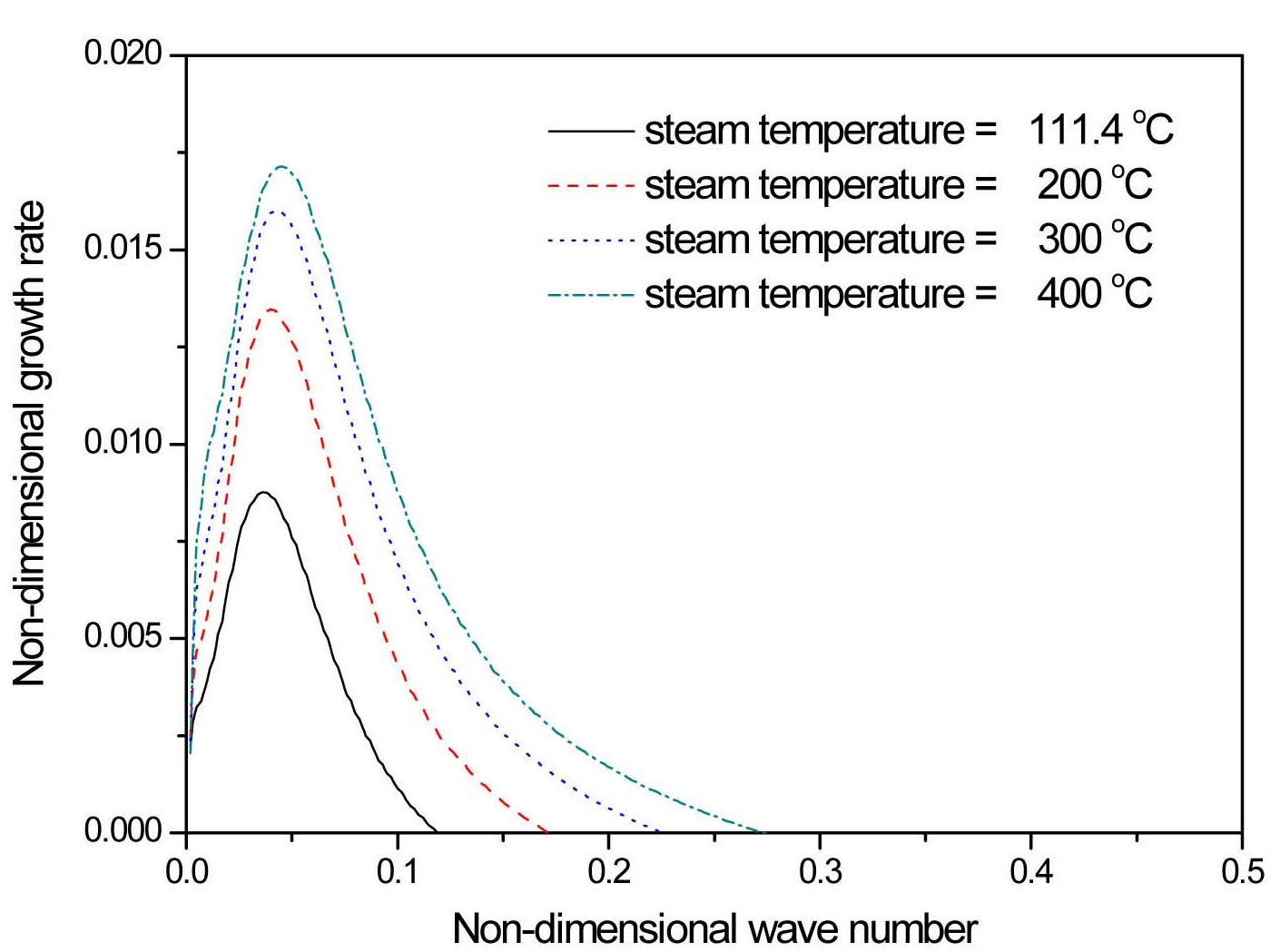
The variation of steam temperature causes changes in the steam properties, and thus water sheet instability. The results in Figure 6 are obtained with a steam temperature change from 111.4 Ū (saturated temperature corresponding to the operating pressure) to 400 ℃. The density and dynamic viscosity of the steam are 0.48~0.86 kg/m³ and 1.27~2.44 N·s/m² in this temperature range, respectively. As steam temperature goes up, the density decreases but the dynamic viscosity increases, which corresponds to a reduction of steam Re number, Re₂. Figure 6 shows that decreasing Re₂ has a destabilizing effect on the water sheet for the selected operating parameters.

Unlike a nuclear fuel rod, the spacer grid structures are unpowered. As a result, their temperatures are much lower than those of the fuel rods. This promotes earlier quenching of the grid structures in comparison to the fuel rods. Once quenched, a thin film is formed on the surface of the grid spacer with sub-cooled or saturated conditions. Figure 7 depicts the temporal growth rate in terms of the wavenumber for several water temperatures which vary from 10 ℃ to the saturated value. The variation of water temperature changes the water properties such as density, dynamic viscosity, and surface tension. The results presented in Figure 7 have destabilizing trends with increasing water temperature. These trends are mainly related to the surface tension effect; its value decreases with temperature. Hagerty and Shea (1955) described that in liquid sheets, unlike round jets, surface tension has a stabilizing effect. Although not shown in the figure, the results without considering the surface tension variation have almost the same graphs with different water temperatures, so the trends in Figure 7 are judged to be mainly due to the surface tension effect. This analysis agrees well with the fact that the characteristics of the spray are almost independent of the liquid viscosity

(Hauke et al, 2001).

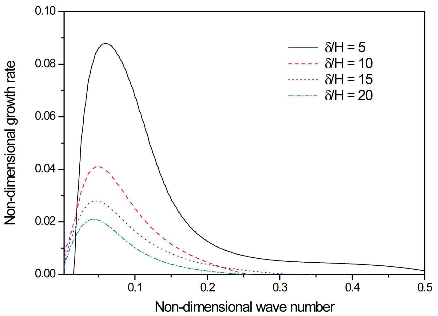
Figure 8 displays the influence of d/H upon the temporal growth rate as a function of the wavenumber, where only the boundary layer thickness for the steam flow is changed, maintaining all the remaining fluid properties and water sheet thicknesses constant. An increase of δ/H is shown to have a stabilizing effect on the water sheet oscillation in the figure; the location for the maximum growth rate shifts to a lower waver number and the range of unstable wave numbers becomes narrower. The thickness of the steam boundary layer has been related to the destabilization of the liquid sheet in terms of vorticity pattern. The thinner the boundary layer, the more vorticity it contains. As the liquid sheet is distorted, the destabilizing pressure fields

induced by the vorticity pattern become stronger (López- Pagés et al, 1999; Hauke et al, 2001; Altimira et al, 2010). The influence of d/H upon the temporal growth rate for the variation of water sheet thicknesses shows a similar trend, although for the sake of clarity the results have not been included in the figure. The increase of water sheet thicknesses, corresponding to a reduction of δ/H, destabilizes the water sheet in such a way that the location for the maximum growth rate shifts to larger wave numbers and the range of unstable wave numbers becomes wider.

The Rod Bundle Heat Transfer (RBHT) test facility was constructed to investigate the flow and heat transfer characteristics within the bundle assembly for the case of LOCA (Hochreiter and Cheung et al. 2010; 2012).To investigate the spacer grid effects on the rod bundle heat transfer, a series of droplet injection experiments have been carried out for a range of constant powers, pressures, inlet sub-cooled droplet temperatures, steam qualities, and inlet steam flow rates with variable droplet injection flow rates. In these experiments, the droplet injection was initiated at various flow rates and the data were recorded for each set of test conditions once a steady-state time period was reached. In addition to the various data channels of temperatures and pressures, droplet data were recorded using a high speed camera system with an infrared laser, i.e., a VisiSizer system. The VisiSizer system, which represents a unique feature of the RBHT facility not found in other rod bundle reflood facilities, consists of a highresolution digital camera, infrared laser, data analysis software, and associated computer and control equipment (Ireland et al., 2003). It is capable of real-time analysis of the droplet size and velocity distributions. From the droplet size distribution measured at a given location, the Sauter mean diameter of the droplets can be determined. The Sauter mean diameters were measured upstream and

downstream of grid spacers #4 and #6 within the RBHT facility at elevations of approximately 1.7 m and 2.5 m, respectively.

Due to the difficulty and uncertainties in velocity measurement using the VisiSizer system, reliable droplet velocity data were not obtained in the steam cooling with droplet injection tests. As such, the droplet data are not sufficient for determining the values of the Weber number. To circumvent this situation, COBRA-TF was utilized to predict the droplet velocities which were missing in the measured data. COBRA-TF input decks were prepared for the RBHT steam cooling with droplet injection tests which provide velocity predictions for the bulk steam flow and the entrained liquid (Miller 2012).

The droplets downstream of the spacer grid consist of initially injected droplets which have not collided with the spacer grid and newly generated droplets from disintegration of the trailing water sheet. Cheung and Bajorek (2011) derived an expression for the ratio of the droplet diameters upstream and downstream of a dry spacer grid by considering the conservation of liquid mass and the kinetic as well as the surface energies. In terms of the diameter, d_gen, of the newly generated droplet group, the following equation can be derived to compare the experimental data with the analytical result:

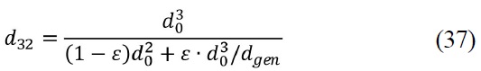
where is the droplet diameter upstream of the spacer grid and is the blockage ratio for the spacer grid. The d_gen values for each test are extracted using the above equation with the Sauter mean droplet diameters measured upstream and downstream of the spacer grid.

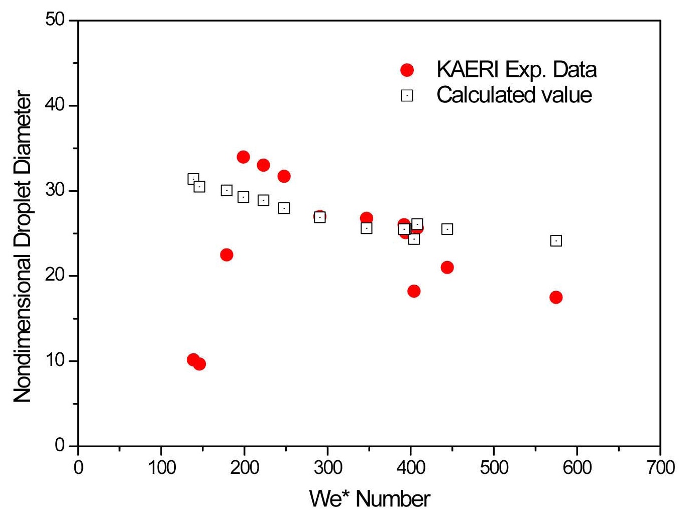
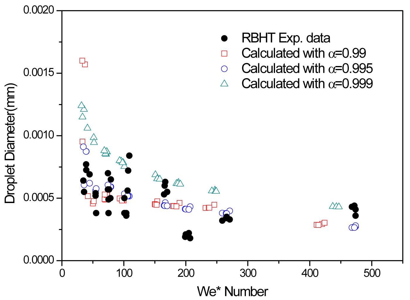
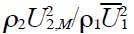
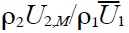
Figure 9 shows a comparison of the predicted drop size as a function of the Weber number with the RBHT data, where the modified Weber number is defined as We^* =

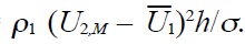
Physically, We^* represents the ratio of the aerodynamic force and surface tension force. The relative velocity concept has been introduced to consider the aerodynamic force of air-assisted type spray in the former studies (Senecal et al., 1999; Sirignano et al., 2000; Sirignano et al., 2010). Considering the results shown in Figure 2 and 3, that the larger steam velocity with lower water velocity has a destabilizing effect on the water sheet, the modified Weber number is judged to reflect the physical mechanism of water sheet breakup better than the original definition based on the water velocity alone. The analytical results are calculated with three different void fractions, 0.99, 0.995, and 0.999. The calculated values show a similar trend as the measured results in such a way that the droplet diameters downstream of a wet spacer grid tend to decrease with increasing Weber number, owing to the reduced film thickness and shorter wave length of the water sheet.

Recently an experiment on the droplet behavior inside a heated rod bundle was performed at Korea Atomic Energy Research Institute (KAERI) (Cho et al., 2011). The experiment focused on the change of droplet size induced by a spacer grid in a rod bundle geometry, which results in the change of the interfacial heat transfer between droplets and superheated steam. The test facility was originally constructed for a reflood heat transfer experiment so that water was supplied from the bottom of the test facility. For the droplet behavior test, the facility was modified so as to provide a steam flow with droplets directly injected into the test section instead of simulating a quench front of reflooding water. The droplet injection nozzle was installed in one sub-channel of the heater rod bundle. A liquid jet break-up method was used for the droplet generation. Droplets were injected into the test section from 0.15m below the grid spacer. The major measuring parameters of the experiment were the droplet size and velocity, which were measured by a high-speed camera and a digital image processing technique. A series of experiments were conducted with various flow conditions

of steam injection velocity, heater temperature, droplet size, and droplet flow rate. Data on the change of the Sauter mean diameter of droplets after collision with a wet grid spacer were obtained for various flow conditions.

The predicted non-dimensional droplet diameters as a function of the modified Weber number We^*, are compared with KAERI data in Figure 10, where the droplet diameters are non-dimensionalized with half water sheet thickness, h. In this experiment, all the injected droplets collide with the spacer grid, so the measured droplet diameters downstream of spacer grid are from the disintegration of the water sheet. As a whole, the non-dimensional droplet diameters display a monotonously decreasing trend with We^*, which means that the most unstable wavenumber displaces to a larger value with an increasing steam flow rate. At a very low We^*, only the experimental data shows a steep increase of the non-dimensional diameters. Ignorance of the varicose oscillation mode or the temporal instability approach of this study are judged to cause the discrepancies of the droplet diameters at a low We^*.

A viscous linear temporal instability model of a water sheet issuing from the trailing edge of a wet spacer grid with a surrounding steam up-flow has been developed to investigate the water droplet generation from a wet grid spacer. Both water and steam were considered viscous and incompressible over the range of operating conditions under consideration. To account for the aerodynamic effect of the surrounding steam flow on the water sheet oscillation development, interfacial boundary conditions correctly reflecting the real situation, including pressure and viscous stresses in balance with surface tension forces, have been formulated. The governing equations have been solved using Chebyshev series expansions and the Tau–Galerkin projection method. Based on the results of this study, the following conclusions can be made:

1. As the steam velocity increases, the unstable region broadens, the maximum growth rates notably increase and their location are displaced toward larger wave numbers, which evidently shows the strong destabilizing effect of the steam velocity on the water sheet. The result for the water velocity variation shows an opposite trend in such a way that the maximum growth rate decreases as the water velocity increases. The non-dimensional frequency and wave propagation speed are practically insensitive to changes in the steam velocity, whereas the wave propagation speed exhibits a decreasing trend with increasing water velocity.

2. As the system pressure goes up, the maximum temporal growth rates are displaced toward larger wave numbers, resulting in a shorter wave length and smaller droplet diameter, while the unstable regions become narrower. If the pressure is larger than 0.3 MPa, the new local peaks emerge at larger wave numbers and grow with the pressure increment.

3. As the steam temperature goes up, the density decreases but the dynamic viscosity increases, which corresponds to a reduction of steam Re number, Re2. Decreasing Re2 is found to destabilize the water sheet for the selected operating parameters. The plots with higher water temperatures also exhibit destabilizing trends, mainly owing to the reduction of surface tension. This result agrees very nicely with previous studies on spray and atomization.

4. A larger δ/H has a stabilizing effect on water sheet oscillation for both cases, a larger δ with constant H and a smaller H with constant δ. This tendency can be explained in terms of vorticity patterns, namely, the thinner the boundary layer, the stronger the destabilizing pressure field induced by the vorticity pattern.

5. Results predicted by the present model have been compared against the RBHT droplet data over a range of modified Weber numbers, We*, representing the ratio of the aerodynamic force to the surface tension force (Srinivasan, 2010). The calculated values show the same trend with the measurement in such a way that the droplet diameters downstream of a wet spacer grid tend to decrease with an increasing Weber number. The predicted non-dimensional droplet diameters also show reasonable agreement with the KAERI data (Cho et al., 2011).

a₀, a₂ coefficients for the velocity profile of water sheet

A₀, A₂ coefficients for the non-dimensional velocity profile of water sheet

b₀, b₁, b₂ coefficients for the velocity profile of surrounding steam boundary layer

B₀, B₁, B₂ coefficients for the non-dimensional velocity profile of surrounding steam boundary layer

a_n, b_n, c_n, d_n, e_n, f_n coefficients for Chebyshev polynomials

C coefficient for the inviscid solution of the outer steam flow

D_H hydraulic diameter of the unit cell, m

d_lig diameter of the cylindrical ligament formed from primary breakup of water sheet, m

d₃₂ Sauter mean diameter of the droplets formed downstream of the wet grid, m

d₀ droplet diameter upstream of the wet grid, m

d_gen droplet diameter newly generated from water sheet breakup, m

g acceleration due to gravity, m/s²

H_film thickness of the liquid film on the surface of the spacer grid, m

h half thickness of water sheet, m

i imaginary part of complex number,

k wavenumber, m^-1

non-dimensional wavenumber

k_max wavenumber corresponding to maximum growth rate, m^-1

l ratio of steam boundary layer to half thickness of water sheet, δ/h

N₁, N₂ largest degree of Chebyshev polynomials

n degree of Chebyshev polynomials

p pressure, N/m²

p' perturbed pressure, N/m²

Re Reynolds number, Re =

R_ke kinetic energy ratio,

R_mo momentum ratio,

t time, s

T_n n^th degree Chebyshev polynomial

U basic velocity in x direction, m/s

Ũ non-dimensional basic flow velocity in x direction

average velocity of water sheet basic flow in x direction, m/s

U_2,M median velocity of surrounding steam flow in x direction, m/s

V₁₂ velocity ratio,

u, v velocities in x, y directions, m/s

u', v' perturbed velocities in x, y directions, m/s

We Weber number,

We^* modified Weber number with steam velocity,

x, y coordinates, m

x,

non-dimensional coordinates

non-dimensional coordinate for the surrounding steam flow

Greek symbols

α void fraction

Δ (2/3) μ_r + l

δ thickness of surrounding steam flow boundary layer, m

η^± upper and lower interface displacements from the equilibrium position, m

η₀ amplitude of the interface displacement, m

non-dimensional amplitude of the interface displacement

λ_max wavelength of corresponding to k_max, m

λ_lig dominant wavelength for the breakup of cylindrical liquid ligament, m

μ dynamic viscosity, Pa-s

μ_r viscosity ratio of steam to water, μ₁/μ ₂

ρ density, kg/m³

ε blockage ratio

σ surface tension, kg/s²

ψ stream function, m²/s

φ amplitudes of the normal mode disturbances, m²/s

non-dimensional amplitudes of the normal mode disturbances

second derivative of

τ_i interfacial stress between surrounding steam and film flows, N/m²

ν kinematic viscosity, m²/s

ω complex frequency, ω_r + ω_i, m^-1

non-dimensional complex frequency

Subscripts

α phase index

1 water

2 steam