Ideally, an electricity supply should invariably shows a perfectly sinusoidal voltage signal at every customer location. However, for a number of reasons, utilities often find it hard to preserve such desirable conditions. The deviation of the voltage and current waveforms from sinusoidal is described in terms of the waveform distortion, which is often expressed as harmonic distortion.
Harmonic distortion constitutes one of the main concerns for engineers in the several stages of energy utilization in the power industry. In the first electric power systems, harmonic distortion was mainly caused by the saturation of transformers, industrial arc furnaces, and other arc devices like large electric welders. The increasing use of nonlinear loads in industry is continuing to increase harmonic distortion in distribution networks. Nonlinear loads include static power converters, which are widely used in industrial applications in the steel, paper, and textile industries. Other applications include multipurpose motor speed control, electrical transportation systems, and electric appliances [13].
The focus of this study was to model a power network using ATP and its graphical processor ATP-Draw [3], in order to study the propagation of harmonics through the power network. This software offers many possibilities based on models [10], where electrical components such as transmission lines, cables, and transformers can be easily modeled. The results obtained by ATP such as currents and voltages can be easily drawn by PlotXY software [12], which also can calculate the Fourier transformation.
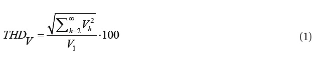
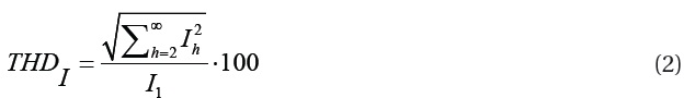
The power network represents an industrial plant, which contains different types of electric components and a harmonic source (3rd, 5th, 7th, 9th and 11th harmonic currents). The simulation of the harmonics propagation will be done to find out the distorted curves of the currents and voltages in different branches of the electrical system, and will be made to control the THD (Total Harmonic Distortion). The standards established in the 1992 revision of IEEE-519-1992 must be adhered to. THD for voltages and currents are calculated as follows [6]:
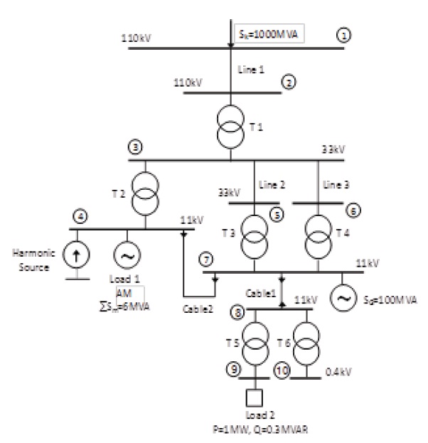
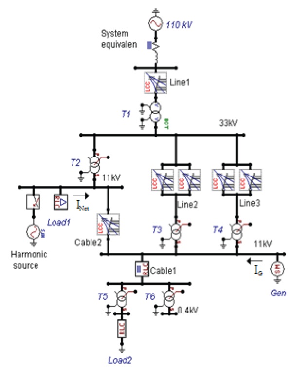
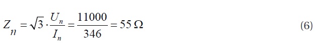
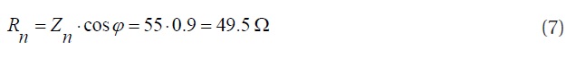
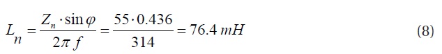
The studied case (Fig. 1) corresponds to a part of a power network, which represents a medium-size industrial plant with 10 buses. On the 110 kV bus (①), the system has a short-circuit power SK"=1,000 MVA. To 11 kV bus (⑦) is connected a synchronous generator with a nominal power of about SG=100 MVA. To the other 11 kV bus (④) is connected an electrical load, which includes a group of asynchronous motors with a total rated power of about Sm=6 MVA, an electric current consumption of about 346 A, and a power factor of 0.9. To the same bus (④) is connected the harmonic source, which injects 3rd, 5th, 7th, 9th and 11th harmonic currents. The network also contains another load at the bus (⑨) equivalent to the load of some streets. The network also has 6 transformers, two cables, and three transmission lines. The data of the network are described in the tables below.
ATP-Draw [3] has several models of transformers, cables, transmission lines, loads, and electric components used in the study of power quality. The calculations carried out and methods used to build the models to simulate the harmonic distortion of currents and voltages are described.
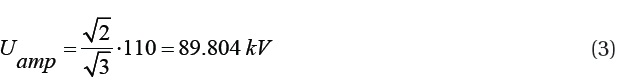
The supply network is represented by voltage source with an amplitude equal to equation 3 [14]. Its internal impedance (R=1.2 Ω, L=38.2 mH) is calculated from the short-circuit power SK". The model of the supply network by ATP-Draw was AC3ph-type 14 (Steady-state (cosinus) function, 3-phase).
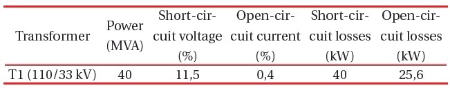
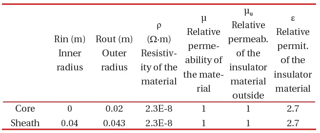
ATP-Draw is able to generate the parameters of transformers from the nominal label values by the built-in procedure BCTRAN, but if the data about transformers is not available, a transformer model SATTRAFO (3phase, Y-Y) can be used, because this model of transformers consists of simple series R and L components, which are variables, and the other values are for all of the transformer constants [1]. For better illustration of ATP-Draw, the transformer T1 will be modeled by BCTRAN and regarded as a distribution substation transformer. The rest of them are regarded as distribution transformers [9] and will be modeled by SATTRAFO. Table 1 describes the parameters of transformer T1 and Table 2 describes the parameters and recommended values for the use of the SATTRAFO transformer model.
The other values: number of phases: 3, windings: 2, shell core, test frequency: 50 Hz, connections: Wye-Wye (voltage is divided
[Table 1.] The parameters of the generator.
The parameters of the generator.
[Table 2.] Constant values for SATTRAFO.
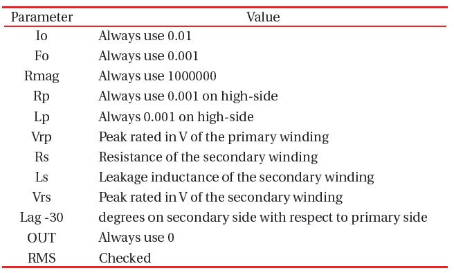
Constant values for SATTRAFO.
by √3).
To use the SATTRAFO model the values Vrp, Rs, Ls, and Vrs are the only variables. The lag variable remains at 30 degrees, because all transformers to be used are D-Y. Series R and L values must be taken at the secondary side of the transformer. As an example, only the calculations for transformer T2 will be used. As shown in Table 3, the specifications of this transformer are 15.7 MVA and 33/11 kV, with an impedance of 15%. All R and L values will be referenced from the secondary-side of the transformer. The secondary-side voltage is 11 kV; therefore:
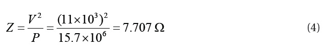
where Z is the impedance, V is the secondary side voltage (11 kV), and P is the power (15.7 MVA).
[Table 3.] The recommended values of variables.
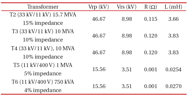
The recommended values of variables.
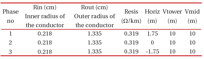
[Table 4.] The parameters of the transmission line 110 kV.
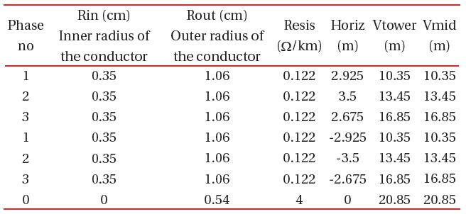
The parameters of the transmission line 110 kV.
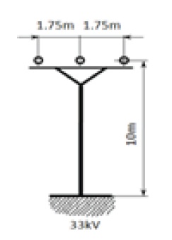
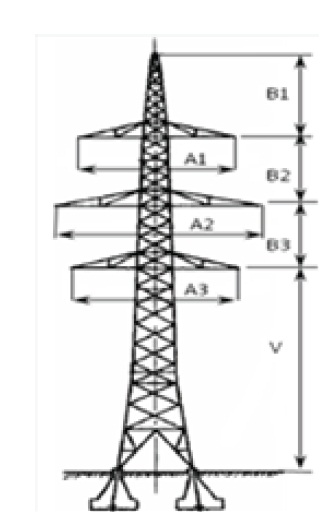
[Table 5.] Dimensions of the tower 110 kV.
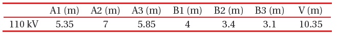
Dimensions of the tower 110 kV.
15% of 7.707 W is 1.156 W. This represents the magnitude of Z, or |R+jX|. A common X/R ratio for transformers is 10 [1,7]. Using this value, it is found that X=10 R. From the equation
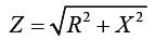
[13], R=0.115 Ω and XL=j1.15 Ω can be calculated. The inductive reactance is XL=jωL, so using a power system frequency of 50 Hz, the inductance is L=3.66 mH.
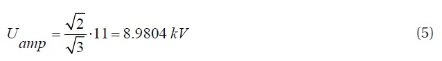
The primary voltage is 33 kV-D. Therefore, the peak primary rated voltage [14] is Vrp=√2×33 kV=46.669 kV. The secondary voltage is 11 kV-Y, so the peak Vrs=√(2/3)×11 kV=8.9815 kV.
Similar calculations were carried out for all transformers. Values are listed in Table 3.
3.3 Transmission lines and cables
Usually, transmission lines and cables can be represented by a resistance R and the reactance X, which can be determined from industrial catalogues or calculated. The ATP-Draw gives many advantages in how to build the transmission line and cable model, which can be done easily by the RLC parameters, or by the built-in procedure Lines/Cables (LCC), which generates the parameters of the element from the input dimensions and material constants.
- The 110 kV transmission line is made of 240AlFe6+earthing 185Fe, with a length of 50 km, and was modeled by the LCC Lines/Cables procedure as an overhead line. 3-phase Bergeron type and was taken into consideration for the skin effect, but the sag was not considered, so Vtower=Vmid. ρ (ground resistivity)=20 Ωm, Freq. init=50 Hz. The parameters are in Table 4. The placement of conductors on the tower is shown in Fig. 2, and the dimensions of the tower are in Table 5.
[Table 6.] The parameters of the transmission line 33 kV.

The parameters of the transmission line 33 kV.
[Table 7.] The parameters of the cable 1 by RLC3 (material: Cu; length= 5 km).

The parameters of the cable 1 by RLC3 (material: Cu; length= 5 km).
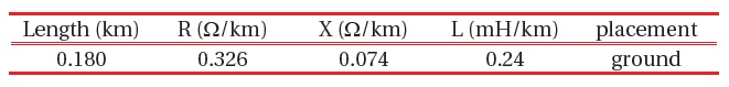
The parameters of cable 2 by lines/cables LCC (3 phase, PImodel, ground, ρ=20 Ω.m, f=50 Hz, length=3 km, total radius=0.045 m, position: vert=0.7 m, Hor=0).
[Table 9.] The parameters of the generator.

The parameters of the generator.
- The transmission line 33 kV is made of 2×AlFe6, 95 mm2, length 5 km and was modeled as the same as the previous with PI-Model. ρ (ground resistivity)=20 Ωm, Freq. init=50 Hz. The parameters are in Table 6 and the placement of the conductors as shown in Fig. 3.
Cables can be simply modeled by RLC3 (3-phase R-L serial circuits), without parallel capacitance. Relatively short-length cables can be treated as pure resistances obtained from the length, area of the core, and resistivity (R=ρ.l/S). The resistance and the reactance are also available in different catalogues and tables. If the parameters of the cable are known, such as the dimensions and material constants, it is suitable to model the cable by the built-in procedure Lines/Cables (LCC). The parameters of two kinds of models are shown in Tables 7 and 8.
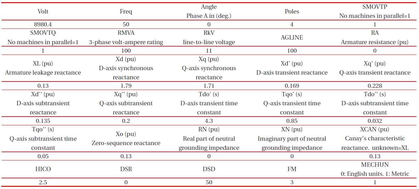
SG of the generator is =100 MVA, operating on the 11 kV bus and can be represented by the SM59 model. This model is offered in ATP-Draw as a synchronous machine, with no TACS control (Transient Analysis of Control Systems), type59, balanced steady-state, and no saturation. The parameters of the generator are listed in Table 9. The voltage magnitude is calculated as in equation 1 and represents the steady-state voltage at the terminals of the machine.
Explanations for Table 9 [10]:
SMOVTP: proportionality factor used only to split the real power among multiple machines in parallel during initialization. No machines in parallel corresponds to SMOVTP =1.
SMOVTQ: proportionality factor which is used only to split the reactive power among multiple machines in parallel during initialization. No machines in parallel corresponds to SMOVTQ=1. Machines in parallel: requires manually input file arranging.
AGLINE: Value of field current in (A) which will produce rated armature voltage on the d-axis. Indirect specification of mutual inductance.
HICO: Moment of inertia of mass. In (million pound.feet2) if MECHUN=0. In (million kg.m2) if MECHUN=1.
DSR: Speed-deviation self-damping coefficient for mass. T=DSR(W-Ws), where W is the speed of mass and Ws is the synchronous speed. In (pound.feet)/(rad/sec) if MECHUN=0. In (N.m)/(rad/sec) if MECHUN=1.
DSD: Absolute-speed self-damping coefficient for mass. T=DSD(W), where W is the speed of mass. In [(pound.feet)/(rad/ sec)] if MECHUN=0. In [(N.m)/(rad/sec)] if MECHUN=1.
FM<=2: Time constants based on open circuit measurements. FM>2: Time constants based on short circuits measurements.
In most cases, the load model does not give the real situation, but in general, the well-known models consist of serial-parallel combinations of RLC (Δ or Y) [5,15]. The load at bus 4, which includes a group of asynchronous motors, was modeled by RLC_ D3 (3-phase R, L and C are delta-coupled). The parameters are calculated as follows without C [14]:
A load can be easily modeled by a standard component RLC_3 (3-phase, same values in all phases) if R, L, and C are known. Assuming that the load at bus 9 consists of a load of some streets and was measured as 1 MW and 0.3 MVAr, for 400 V, the values of the model will be R=U2/P=0.16 Ω, L=(U2/Q)/2 πf=1.6985 mH, and C=0.
[Table 10.] The values of the harmonic source.
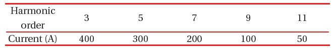
The values of the harmonic source.
The source of harmonics injects (hypothetically) the 3rd, 5th, 7th, 9th, and 11th current (with 0 Angles) to the system. The ATP-Draw library includes only a single-phase harmonic source, so the calculation will be related to phase A. The model of the source is HFS_Sour (Harmonic frequency scan source, TYPE 14). The values of the harmonic sources are usually obtained from field testing, but for illustration, the source was modeled by the hypothetical values in the table below.
To start the simulation, there are some important parameters affecting the simulation. In the menu ATP→Settings, for all simulations, ΔT has been set to 100 ms, and Tmax to 5s. This gives a simulation time of 250 cycles. These cycles are adequate for the simulation time to obtain an estimate of any variations in the voltage and current. The initial time for all figures starts at 4.8s, and the initial time for the Fourier transformation is set to 4.98s. When Xopt is set to zero, all inductances are in mH. Copt: similarly, capacitances are in μF. Freq: System Frequency. This is only used if Xopt or Copt are non-zero, but it is always good practice to set this to the system frequency of 50 Hz.
This study investigates the harmonic voltages at the primary and secondary side of transformers, the harmonic currents through them, and some buses and branches of concern. The ATP-Draw model of the network is shown in Fig. 4.
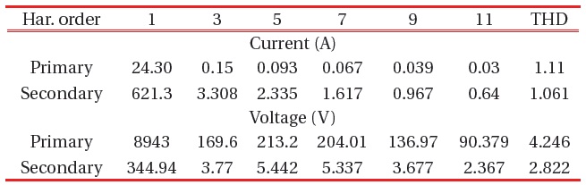
[Table 11.] The harmonic currents and voltages at T1.
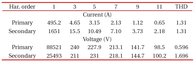
The harmonic currents and voltages at T1.
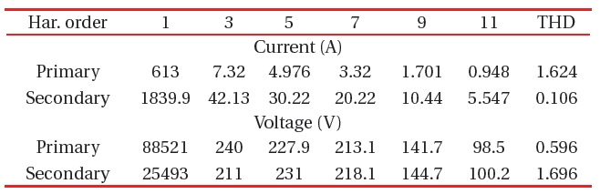
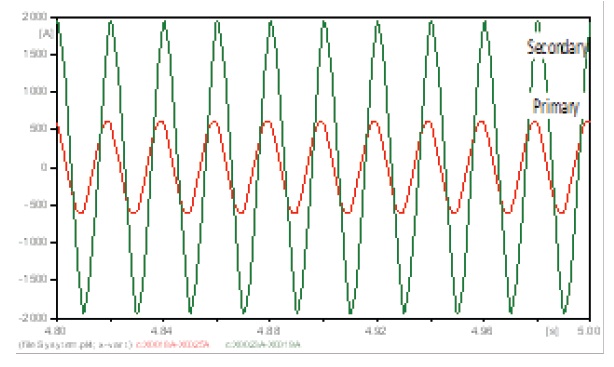
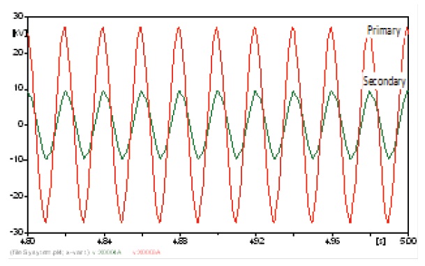
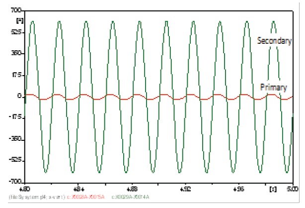
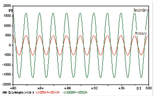
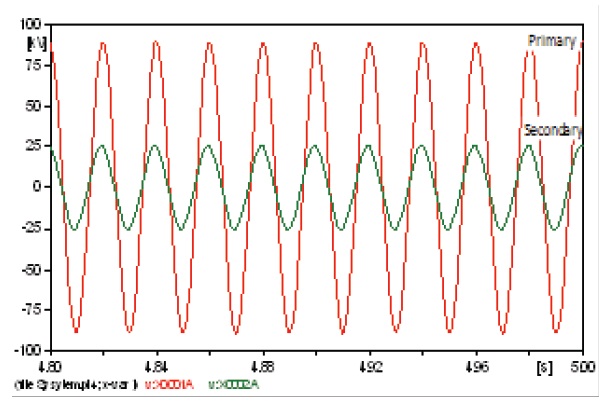
Transformer T1 is far from the harmonic source, so the curves of the currents and voltages have to be sinusoidal, but to some extent, they were affected by the harmonic source. Because transformer T1 was connected with its windings in star-star, the primary and secondary line currents will have the same wave form and the same THD. The primary and the secondary currents are shown in Fig. 5, the primary and the secondary voltages are shown in Fig. 6, and the values of the harmonic contents are listed in the table below for both harmonic currents and voltages.
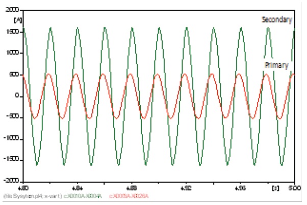
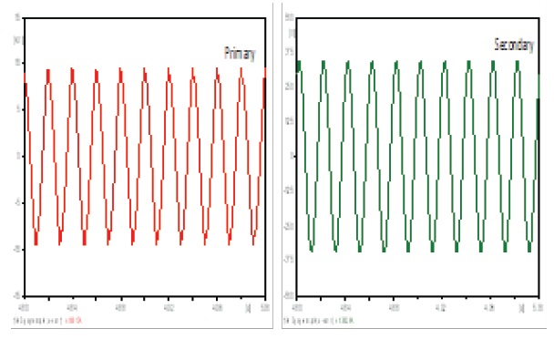
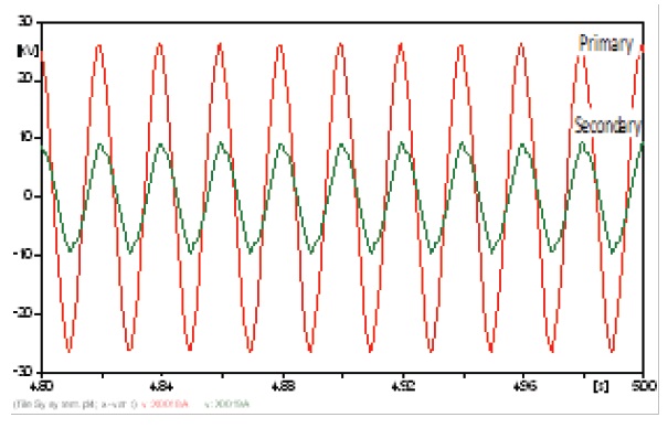
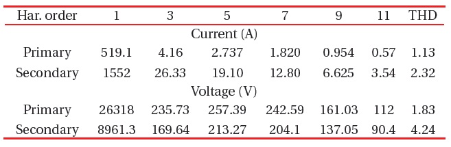
The windings are connected in delta-star, so the secondary current is a phase current, while the primary is a line current, which is a combination of two primary phase currents. This changes their wave form, but not its harmonics content or its THD [15]. The results are shown in Figs. 7 and 8 and the harmonic contents in Table 12.
[Table 12.] The harmonic currents and voltages at T2.

The harmonic currents and voltages at T2.
[Table 13.] The harmonic currents and voltages at T3.
The harmonic currents and voltages at T3.
Transformers T3 and T4 are similar, so the results will be similar too. Therefore, for both of them, the same explanations apply as before (T2), and the results are shown in Figs. 9 and 10 and in the table below (just for T3).
The same explanations as before are applied. The results are in Figs. 11 and 12 and in the table below.
[Table 14.] The harmonic currents and voltages at T5.

The harmonic currents and voltages at T5.
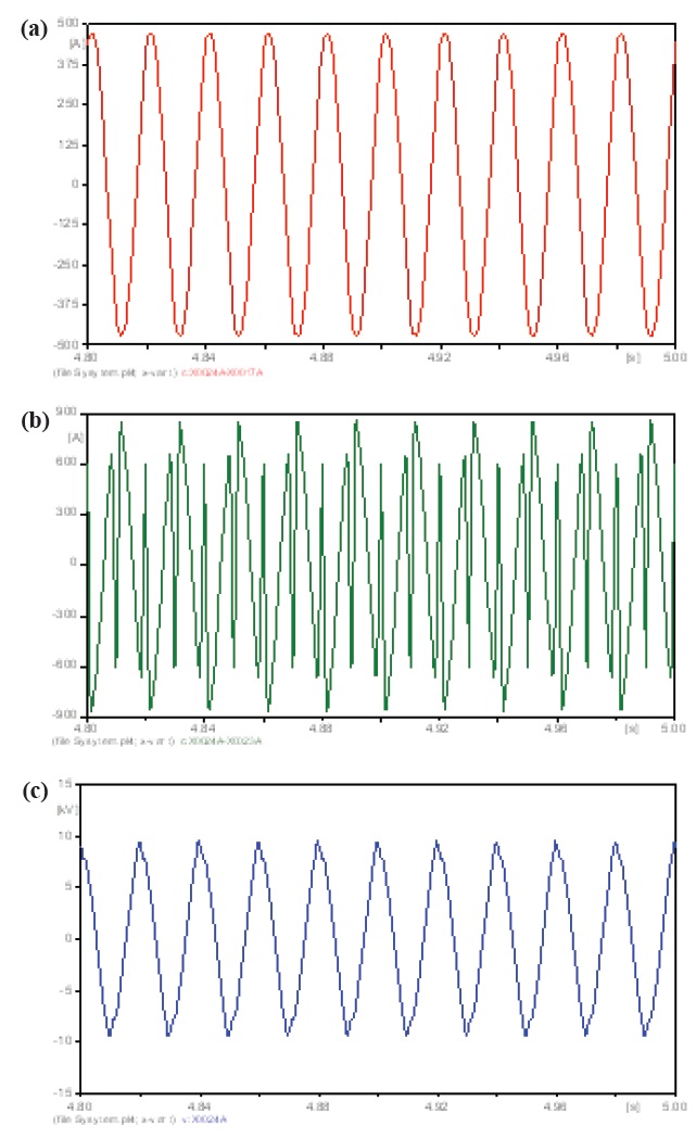
This bus is affected by the harmonic source, which is clearly seen from the wave forms in Figs. 13(a)-(c). The current which
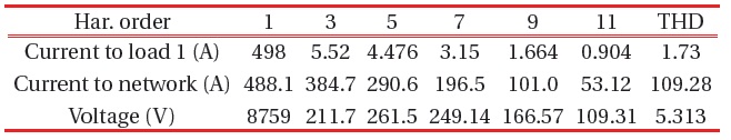
[Table 15.] The harmonic currents and voltage at bus 4.

The harmonic currents and voltage at bus 4.
[Table 16.] The harmonic currents and voltage at bus 4.
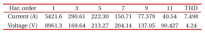
The harmonic currents and voltage at bus 4.
flows to load 1 is a little distorted, but the harmonic currents continue to the network (INet - Fig. 4), and this affects the whole power system and causes a waveform distortion, which is seen in the previous figures. The voltage at this bus is distorted, too. The results are in Table 15.
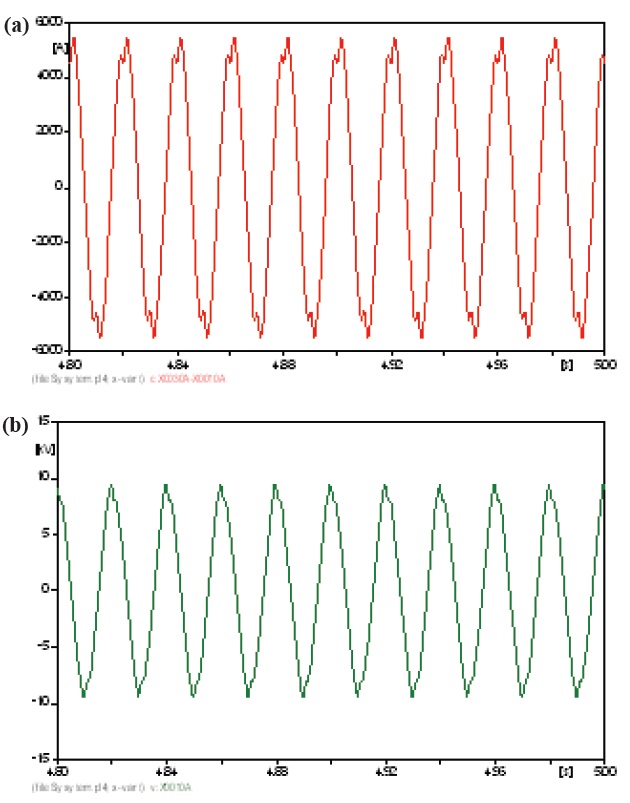
The current that flows from the generator (IG-Fig. 4) has a high distortion, and the voltage at this bus has a high distortion too (Figs. 14(a) and (b)). The results are in Table 16.
The modeling of power system elements can help engineers to find solutions for problems related to harmonics, even with complications about how to find an accurate model for some elements of the power system. With this simple example, the helpfulness of ATP has been demonstrated for harmonics propagation analysis . It is important carefully enter data into the program, because the desired results depend on this data.
The different figures show the propagation of harmonics through the whole electric system, starting from the source of harmonics via different buses to the far end of the network. Some transformers and buses are affected more, and some of them less. The THD of the primary current of all transformers did not exceed 2%, and the secondary current was 3%. The main harmonic was the 3rd harmonic with an amplitude that reached 1.19% on the primary side of T2 and 2.29% on the secondary side. The THD of the voltages reached 4.246% on the primary side of T5 and 5.313% on the secondary side of T2. The main harmonic was the 5th harmonic with an amplitude that reached 2.38% on the primary side of T5 and 2.84% on the secondary side of T2. Both buses 4 and 7 were affected. The voltage at bus 4 had 5.313% THD, and bus 7 had 4.24% THD. The main harmonic was the 5th harmonic with an amplitude of 2.99% at bus 4.
From the knowledge of harmonics propagation, it should be kept in mind that the electromagnetic radiation generated by the sources has to be minimized, and it is advisable to strictly follow the manufacturer’s recommendations, or suitable filters should be installed to reduce the harmonics.