The pipe routing design as it pertains to shipbuilding is usually performed during the basic and detail design stage after the creation of the pipe & instrument diagram (P&ID), which contains connection data between equipment in the preliminary design stage. Generally, this type of pipe routing design is accomplished by a highly experienced designer who can consider not only the complex shapes and connections of each piece of equipment but also the issues of space availability, material costs, accessibility, and suitability for installation. The amount of pipe routing work is nearly a half of all outfitting design work at that stage. In addition, the quality of the pipe routing design effort has a direct effect on the subsequent construction design stage, on which the total material and construction cost strongly depends (Shao et al., 2009), just like other design work in the detail design stage of shipbuilding.

When we consider the Just-In-Time (JIT) production scheme in the area of shipbuilding, not only the quality of the routing design which guarantees an accurate amount of raw materials for pipe construction but also the on-time delivery of the routing result to the subsequent design stage are very important in JIT production (Koenig et al., 2002). Moreover, every ship has different specifications, except for a few sister ships. Therefore, every ship needs to be designed based on individual specifications. Consequently, the ratio of the design cost to the total building cost is significantly higher in the shipbuilding industry. Therefore, pipe-routing design automation schemes with feasible quality results that are delivered on time have been key issues to those seeking shipbuilding design process improvements.

The pipe routing optimization problem should satisfy the various constraints. Park (2002) and Qian et al. (2008) categorized these constraints into the two groups of restrictive constraints and quantifiable constraints. Some of them are discussed below.

Physical Constraints

The pipe routing should avoid physical obstacles and connect to the proper equipment.

Economic Constraints

The pipe routing should minimize the total material and fabrication cost by reducing pipe lengths and number of bent parts and by increasing shared pipe supports.

Operational Constraints

The pipe routing should consider the proper operations like valve accessibility and clearance from some equipment for safety.

Physical and operational constraints are restrictive while economic constraints are quantifiable. Therefore, pipe routing optimization seeks to find the best path from an economic point of view among the set of feasible paths restricted by physical and operation constraints.

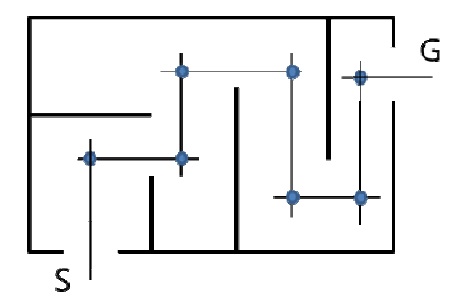
Various types of optimization algorithms have been applied to the pipe routing problem. In an early example, the Maze algorithm was proposed by Lee (1961). This algorithm divides a space into cells and labels and chooses the next cell until the target cell is reached. Hightower (1969) proposed the escape algorithm, also known as the line-search algorithm. This is shown in Fig. 1.

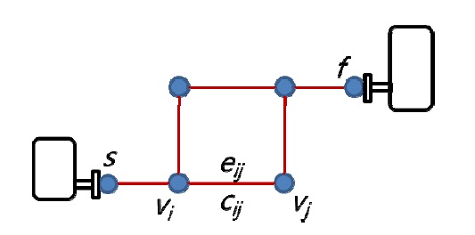
Some network-based algorithms can be used to solve various problems (Nicholson, 1966; Ando and Kimura, 2011). In network-based optimization, each vertex v_i denotes the junction of a pipe where a bent pipe part can be placed; the edge e_ij between the vertexes v_i and v_j denotes a straight pipe part with cost c_ij. Fig. 2 shows a graph representation of this.

In Eq. (1), V denotes the set of vertices, E is the set of edges, and C denotes the cost. The pipe routing optimization problem is to find the shortest path between the start vertex s and the end vertex f in the graph G in Fig. 2. These traditional routing algorithms with graph representation are generally based on what is known as the ‘cell decomposition’ approach. The cell decomposes the problem space containing the start and end points of the target equipment into cubic cells to reduce the problem size and represent the pipe path through the sequencing of connected cells. A good example was given by Asmara and Nienhuis (2006). Ito (1999), Park (2002) and Ando and Kimura (2011) also applied for this approach to represent the pipe routing path.

To find the global optimum route path, several efforts have been made. Examples include an evolution-based algorithm such as a genetic algorithm (Ito, 1999; Ikehira et al., 2005; Kimura, 2011) and an ant colony optimization scheme (Xiaoning et al., 2006, 2007). The target of route optimization is usually the minimum cost of the pipe routing path. In many studies, the cost consists of the pipe length cost and the cost of all bent parts, which require expensive bending fabrication or elbow fitting processes. Park (2002), Kimura and Ikehira (2009) and Ando and Kimura (2011) also considered the operability costs such as the costs incurred to determine valve locations and safety clearances.

Much research has been done since the 1970s. However, there are still limitations when attempting to make use of it to create a fully automatic routing system for actual shipbuilding design work. As discussed by Missuta et al. (1986) and Kang et al. (1999), the main reason for this is that pipe routing algorithms generally do not consider the knowledge and the preference of the designer suitably as required in the actual design work. This type of limitation is not a matter purely related to the optimization algorithm itself. It is rather a matter of knowledge representation during the design automation process (Sriram et al., 1989). Therefore, the knowledge representation in the design has become a more important issue in the area of design automation. Moreover, from a practical point of view, it is also important that the implemented routing algorithm can be utilized effectively in an actual shipbuilding design environment. Some pipe routing algorithms are evaluated in the form of a design support package program; these have a neutral data interface to a CAD system for practical use (Sandurkar and Chen, 1999; Asmara and Nienhuis, 2006; Paulo and Lobo, 2009). They use text-based neutral files such as standard tessellation language (STL) for interfacing data to the CAD system. After constructing the pipe network, Ruy et al. (2012) studied a hole plan system recently.

The pipe routing algorithm developed in this research is based on a network optimization algorithm. The target space including target equipment is divided into non-uniform cells. The graph is constructed considering the route constraints of the fitness of the space, pipe length and bending. This graph represents the pipe route in the target space. An optimum route path can then be obtained by a general minimum path-finding algorithm.

Cell decomposition

Cell decomposition is useful strategy for reducing the problem size. Cell decomposition divides a continuous target space on which pipe lines and equipment are positioned into discrete cells. The edges and vertexes of the divided cubic cells can represent the edges and vertexes of the graph, which connect the start and end points of the routing path. In this case, the network based routing algorithm can be practically applied to these graphs in a reduced problem space. One of the major issues associated with this cell-division method is the number of cells. A larger number of cells generally guarantees a better route path but takes more time to calculate. Therefore, the number of cubic cells should be controlled considering the characteristics of the problems.

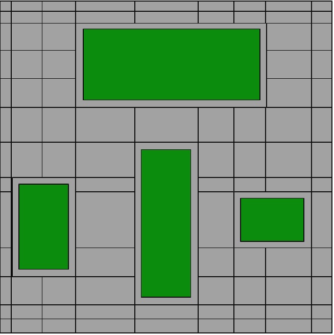
A pipe path along the wall or ceiling structures is preferred due to the issue of space availability after the routing process. This indicates that this near wall space has higher fitness than other spaces. In this research, the target space is divided non-uniformly according to the degree of the special fitness. A space with higher fitness is divided into smaller cubic spaces. The vertexes and edges of cubic cells can be used as the vertexes and edges of the graph which contains a candidate route path. Thus, the space with higher fitness has denser cubic cells and more candidate routes. In contrast, the space around passageways or equipment which may require some distance is divided into larger cubic cell. This cell-division strategy is a part of the consideration of routing design practices pertaining to space fitness. Fig. 3 shows non-uniformly divided cells in the target space. Each cubic cell can have its own fitness factor, and this fitness factor has an effect on the cost decision (value c_ij) between the vertices in Fig. 2.

Graph construction

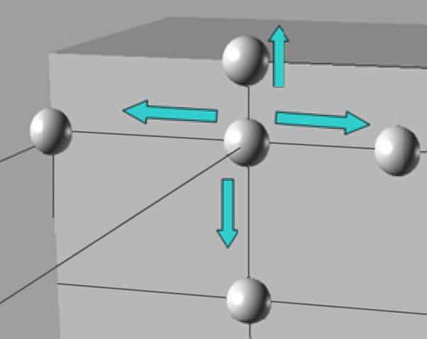
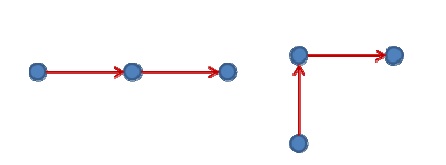
As mentioned above, the vertices and edges of a cubic cell in the target space could be the vertices and edges of the graph. Though the numbers of vertices and edges are reduced by cell decomposition, it is still possible for the graph to be more simplified while maintaining a feasible route path in the target space. To construct a simpler graph, a vertex construction strategy is developed. It is essentially based on the escape algorithm proposed by Hightower (1969). The original escape algorithm is fast and simple, producing one solution directly, as shown in Fig. 3, but it cannot guarantee a solution (Kai-jian and Hong-e, 1987). The vertex construction method of this system uses a strategy similar to that of the escape algorithm to expand the route graph. An edge runs like a beam until it encounters the side of an obstacle or a wall boundary of the target space, at this point it branches off in another direction, as shown below in Fig. 4.

A branch also could be made during edge runs when it meets the edges of cubic cells in the target space. Therefore, a dense area with smaller cubic cells in the target space has more candidate vertices; i.e., it is a preferable space with more candidate vertices.

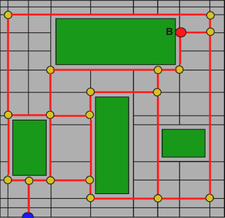
The vertices are located on the corners of non-uniformly divided cubic cells and are connected by edges which have their own weight factor, as shown in Fig. 5. Basically, a network graph is characterized only by the vertices and weighted edges between them. In terms of this traditional definition of a graph, the two graphs in Fig. 6 are equivalent. The relative location of the vertices makes no difference while the connection is maintained.

However, the vertex and edge connection of the graph applied in this system needs to have a topological meaning, as the graph should represent the physical pipe routing. An edge connection running in the target space corresponds to the pipe routing and the vertex on the corner of a cubic cell also contains location information. In this new definition, the equivalent graphs in Fig. 6 are not the same. The figure on the left is a straight pipe and the right side is a bent one. This bending route needs the pipe-bending or an additional elbow fitting pipe part, which generally increases the cost compared to a straight pipe. Therefore, this type of bent pipe should be considered as a cost factor in the route optimize algorithm. To consider a bent pipe such as this one in the graph, a vertex split strategy is introduced. This strategy simply removes the ambiguousness of vertex connections.

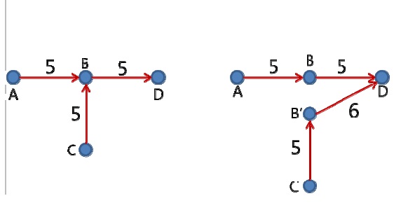
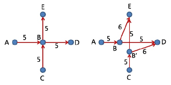
The left figure in Fig. 7 is a part of a route graph with a directional edge, showing each weight factor. In this graph, route AB- D is a straight route while route C-B-D is a bent one. However, the edge between B and D also has a single weight factor of 5; it can be part of A-B-D and part of C-B-D at the same time. Therefore, a pipe bent in this manner is not suitable for this type of graph structure. The right graph of Fig. 7 illustrates the vertex split strategy. Vertex B is split into B and B’ with a bending penalty weight factor of 6. The graph is reconstructed with route A-B-D and route C-B’-D. Then, the bending of the route could be considered without ambiguity.

A vertex with two or more incoming edges and outgoing edges should be split when outgoing edges can be used in a different route path, straight or bent simultaneously. In the case shown in Fig. 8, there are two split vertices. Practically, in a 3D cubic cell space where the number of neighbor vertices cannot exceed six, the number of split vertices is at most three in a case with three incoming edges and three outgoing edges.

Fig. 8 shows another example of a vertex split. This vertex split strategy expands the route graph for mapping onto an actual pipe route in the target space considering the relative locations of the neighbor vertices. The weight factor of an edge is proportional to the penalty factor expressed by Eq. (2), which is evaluated according to the distance and space factor of the edge location and the bent condition.

Eq. (2) accounts for the component of the weight factor, the distance is the actual distance between two vertices, and the distance factor adjusts for the effect of the distance in the weight factor. The bending factor has a positive value when an edge is a part of a bent route. On the other hand, the space factor shows the fitness of the space; here, a smaller value means better fitness. For example, a cubic cell located near equipment, a wall or a ceiling has a smaller space factor because it is a preferable space.

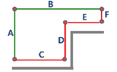
Routes A-B and C-D-E-F in Fig. 9 have the same distance. If the space factor (a route along wall is recommended generally recommended) is more important than the bending factor, route C-D-E-F would be chosen; otherwise, route A-B with less bending would be selected by the optimization algorithm.

Shortest path-finding algorithm

After the vertex distribution and weight decision of the edges, the path-finding algorithm to find the shortest path for the graph can be applied. The shortest path of the graph may be the best pipe route because the weights of the edges represent the total cost of the route, including the materials, fabrication cost, operation cost, and other factors. The graph constructed with these rules is a directional and positive single graph. Therefore, Dijkstra’s algorithm can be applied. For the simplest implementation, it is known that the running time of Dijkstra’s algorithm is in O(V²). Therefore, the construction of the simpler graph G is an important process in the development of this automatic routing scheme. The non-uniform cell decomposition and the vertex location strategy can reduce the size of the graph considerably as well.

The sizes of the non-uniformly divided cubic cells and the edge weight factors are all based on the practices of the pipe routing designer. This practice should be represented and controlled explicitly in the system to be used by a designer who may not have enough pipe routing experience or who wants to accomplish the pipe routing tasks quickly.

In this development, the design practice is basically represented as a parameter. Some aspects, such as the wall side preferences, can be represented by a parameter set that affect the fitness of the space near the side wall, while other practices such as grouping pipes on the same pipe support cannot easily be represented by a parameter set. Therefore, the former is represented in the form of a parameter set and the latter remains as work needing to be done by the designer, who can review and modify the automatic routing result.

The parameters are classified into two groups, one for cell decomposition and the evaluation of the space fitness, and the other for the construction of an efficient graph. The designer can choose a pre-defined parameter set or modify each parameter depending on their preferences. It should be noted that this approach cannot cover all tasks needed for the full automation of the pipe routing routine. Further studies are necessary to accomplish this. Note that a rapid design cycle including automatic routing and route modification, however, can still be practically accomplished.

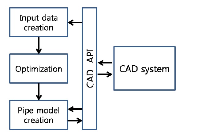
The automatic routing system consists of three modules. The first module is for input data creation, the second one is for routing optimization, and the third one is for the resulting pipe model and for its modification. The input data module and pipe model creation module are embedded in the CAD system Tribon M3 of AVEVA Marine Design and Engineering, while the routing optimization module is a standalone program.

This CAD system provides an application program interface (API) written in Python script. Therefore, the main structure of this automatic routing system is written in Python and the mathematic library and GUI are written in C++. These two embedded modules exchange data with the CAD system directly via the API and the standalone optimization module receives and sends data via the XML file format. Fig. 10 presents the configuration of the automatic routing system.

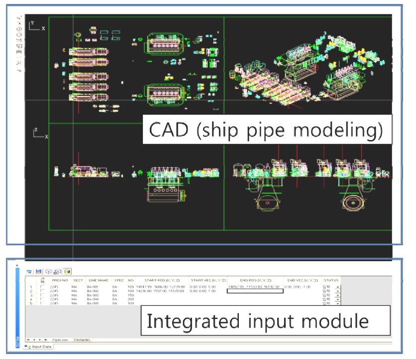
The input data creation module obtains the equipment connection data from the P&ID and the equipment property data from the CAD database. It also has a user input interface with which the designer can input or modify the space and equipment data. This module generates cell decomposition data and equipment data and sends this data to the routing optimization module. The equipment volume is simplified as a cuboid and the locations of the pipe connections on the equipment are modified depending on the direction of the flow for practical reasons. The target space is divided non-uniformly according to the space fitness and the equipment volume is then subtracted. Fig. 11 shows the input data creation module integrated in the CAD system. The designer can select and change the parameter set as they wish, and this selected parameter set governs the routing result.

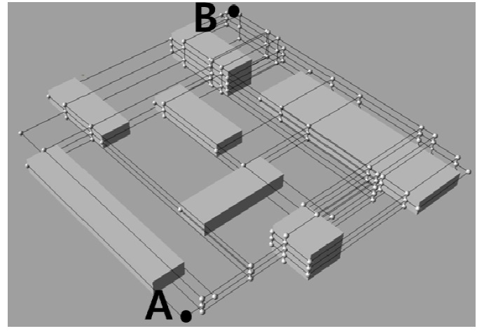
The route optimization module divides the target space non-uniformly and constructs a network graph with the vertex and edges of the cubic cell. Fig. 12 shows an example of a constructed route path graph with start point A and end point B.

This module creates an actual pipe model in the CAD system with the routing result from the optimization module and the pipe specification data from the input data module. This module runs on the pipe modeling CAD system. Thus, the designer can modify or confirm the pipe model in the same user environment.

This module also generates the pipe model data for the following stage of production, including the design and preparation stages. One of the most important types of model data is the bill of materials (BOM), which contains information about the raw materials and the construction processes. The BOM of this system would be accurate and on time because it is based on the accurately and quickly created pipe model. This feature of the BOM plays an important role in the JIT production processes.

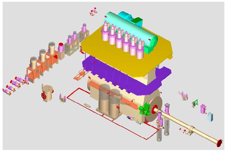
This automatic routing system is applied to pipe routing in a ship engine room space. The volume of the engine and some equipment in the target space are shown in Fig. 13.

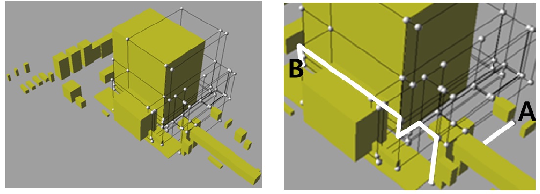
The left side in Fig. 14 shows a simplified graph of the equipment volume and candidate pipe routing. The graph is constructed according to design as represented by the parameters. The right side in Fig. 14 shows the routing result from the start A to end B points.

This system can produce a practical pipe-routing result, showing the amount of pipe material and the approximate route path information. This type of information is useful during the basic design stage. However, this auto-routing pipe model should be checked whether detailed pipe routing practices and rules are considered. These considerations include the air pockets, the thermal expansion, the alignment of support structures, and the valve accessibility, for instance, at the detail design stage. Moreover, some path modification is necessary to utilize the extra space caused by the cuboid simplification of the equipment volume and to reduce the degree of complexity in the narrow spaces through the use of diagonal piping and bent pipes instead of elbow fittings.

In an actual pipe routing job in a shipbuilding outfitting design, there are numerous pipe lines in a single work area (e.g., a block, a room); moreover, there are not only simple pipes which have single start and end point but also pipes with bypasses or branches. This system can handle multiple pipes via the input data creation module, and the automatic pipe routing is done sequentially. Therefore, the sequence set by the designer in the input data creation module characterizes the total routing result of multiple pipes. And this system can handle only simple pipes, the pipe lines with bypass or branch should be divided into simple one in the input data creation module.

A practical automatic pipe routing system is developed and integrated in a shipbuilding CAD system. The pipe routing algorithm is based on graph optimization. A graph containing candidate route paths is constructed on a target space composed of ununiformly divided cubic cells. The design preferences are represented and managed by parameters.

This system is applied to the engine room area of a commercial ship. The result shows that the system cannot always produce the best pipe route initially. However, the designer can recalculate the result easily and quickly with a new parameter set to obtain a satisfying result in the integrated CAD environment. However, there are several limitations of this system. These are mainly related to the management of design knowledge and practices which are rarely expressed by a simple parameter. However, the routing result can serve as a good basis for data generation tasks such as the creation of a BOM and for detailed pipe routing with slight modifications. As a result, the lead time of the basic pipe design stage can be reduced and more accurate and earlier product model data can be produced. These features of the system can improve the productivity of outfitting design and construction in the shipbuilding industry.