Fr Froude number [-]
g Gravity acceleration [m/s]
L Length of the model [m]
N Number of particle image pairs [-]
Re Reynolds number [-]
U Towing speed [m/s]
un Instantaneous velocity of n-th velocity field [m/s]
u x-directional component of mean velocity [m/s]
v y-directional component of mean velocity [m/s]
w z-directional component of mean velocity [m/s]
α Magnification factor [mm/pixel]
Δt Time interval between two laser pulses [s]
ΔX Displacement on particle image [pixels]
μ Dynamic viscosity of fresh water [kg/m·s]
ρ Density of fresh water [kg/m3]
Detailed information on the free-surface wave flow in the turbulent wake of a surface-piercing body is critically important in (1) designing ship hull forms for better propulsion and maneuvering performance, (2) assessing structural reliability of piers, and (3) floating structures’ damping motion in response to external forces, etc. To observe physical phenomena around the surface piercing body, several experimental and computational studies were carried out. Pogozelski et al. (1997) performed velocity measurements near the free surface of a surface piercing body with an early day PIV system and observed wave breaking and boundary layer separation. With the separation, generation of longitudinal vortices was observed where the shoulder wave breaks. Zhang and Stern (1996) and Kandasamy (2001) computed free surface waves around a surface piercing NACA 0024 hydrofoil with a Reynolds averaged Navier Stokes (RANS) solver and simulated the phenomena in the separated flow region at various advancing speeds. Metcalf et al. (2006) investigated boundary layer separation around NACA 0024 foil in various Froude numbers by measuring the surface pressure on the model and free surface elevation, and suggested the unsteady PIV measurement as future work. Based on the measured data, Xing et al. (2007) and Kandasamy et al. (2009) validated their computational fluid dynamics (CFD) codes. The flow around circular cylinders, as well as hydrofoils, is another major concern in surface piercing object problems since it contains unsteady vortex shedding. Inoue et al. (1993) measured time averaged free surface elevation. Flows around surface piercing bodies including a hydrofoil and circular cylinder were simulated using an unsteady RANS solver with volume of fluid method by Rhee (2009). In addition, hydrodynamic interaction of cylinder array with incident wave was calculated by Park et al. (2010).
PIV, as stated above, is one of the most effective methods to investigate flow fields around a surface piercing object because improvements of computer performance in recent years enabled processing of numerous image data to analyze precise vector fields. Since plentiful experimental results were drawn by the application of PIV technique, attempts to introduce a PIV system into a towing tank were materialized. Unlike other hydrodynamic experiments in circulating water channels and cavitation tunnels, towing tank tests are free from blockage effects and free stream turbulent fluctuations in the flow. Thus, towing tank PIV systems have many advantages for tests of turbulent flow including the free surface. Gui et al. (2001) reconstructed the three-dimensional (3D) nominal wake of a combatant using 2D data and compared with the results of five-hole Pitot tube measurement with uncertainty assessment. Uncertainty assessments for towing tank PIV system and other measurement instruments were also executed by Longo and Stern (2005). In addition, Longo et al. (2007) measured nominal wake of a surface combatant model in head seas with 2D PIV in a towing tank and Yoon (2009) measured the flow field around a surface combatant in planar motion mechanism maneuvers with a stereo PIV system and compared with the results of CFD studies. Besides the nominal wake, the flow fields in propeller open water test were measured by Anschau and Mach (2007) with underwater stereo PIV.
In the present study, a towed underwater PIV system was tested in a towing tank and used to investigate the free-surface effects on the turbulent wake of a simple surface-piercing body, and the experimental results were organized to be used as validation data for CFD simulations. In this paper, the description of the PIV system and test model is given in the next two sections. Then uncertainty assessment is explained, followed by the experimental results, discussion and conclusions.
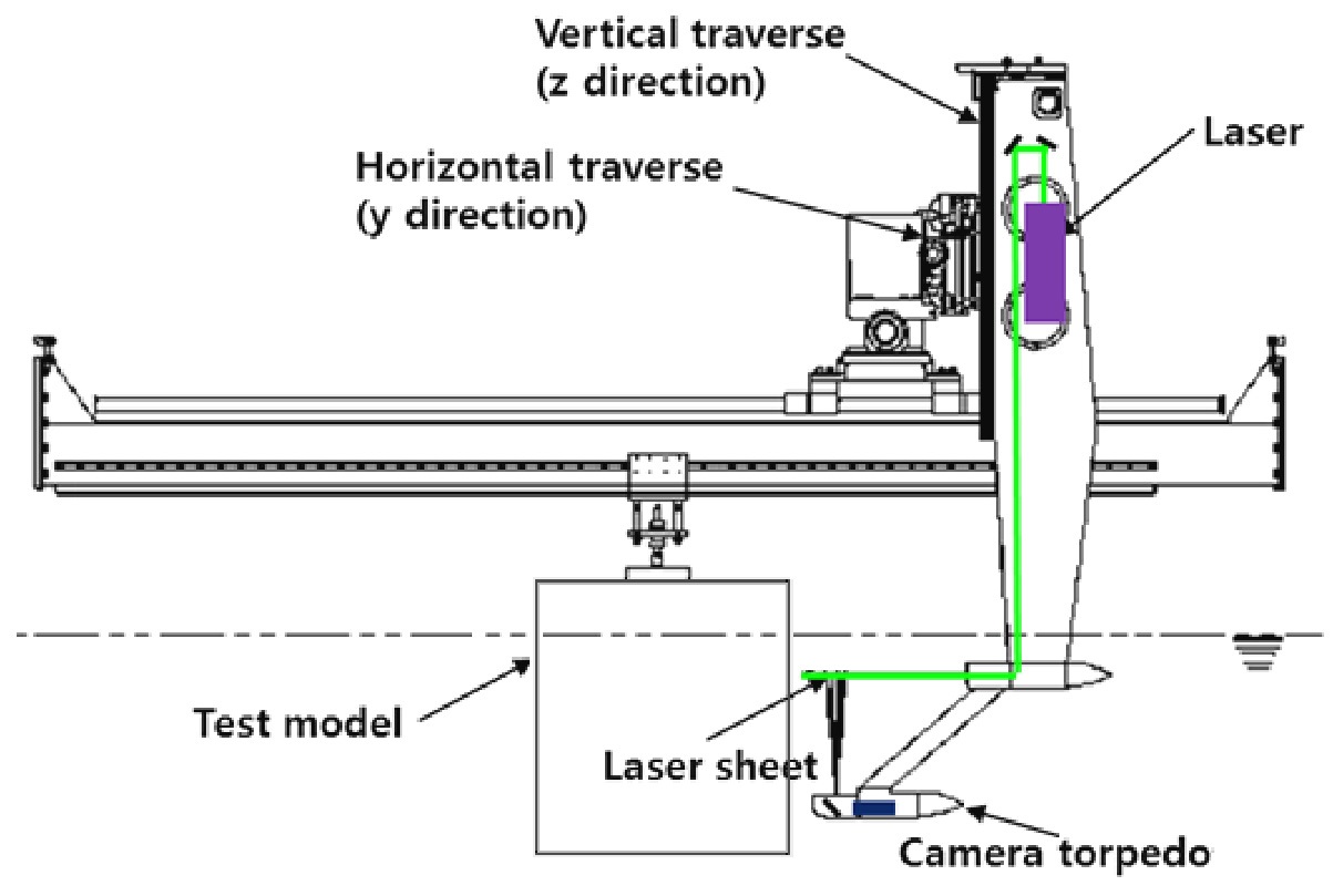
The PIV measurements were conducted in the Seoul National University towing tank, which is 110 m long, 8 m wide and 3.5 m deep. The PIV system consisted of 50 mJ dual Nd:Yag laser (pulse rate: 15 Hz per each laser head) and a 1,600 × 1,200 pixel digital camera fitted with a NIKKOR f/1.4 50 mm lens. The corresponding field of view was 102.08 mm × 76.56 mm. Optical lenses to make the laser sheet and the camera module were placed in a waterproof case. Fig. 1 is the schematic diagram of the PIV system. The waterproof cases are in streamlined shape to minimize the interference in the flow field.
Polyamide powder with a density of 1,030 kg/m3 and an average diameter of 27 μm was used for tracer particles. For particle seeding, a specially designed pressurized seeding tank was used. The seeding was conducted before each test run. The pulse power of the laser head was set as 40 mJ. The DANTEC measurement software, Dynamic studio V2.2, was used to capture the particle images and analyze the velocity fields.
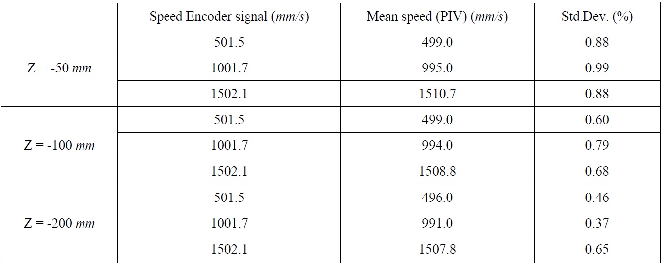
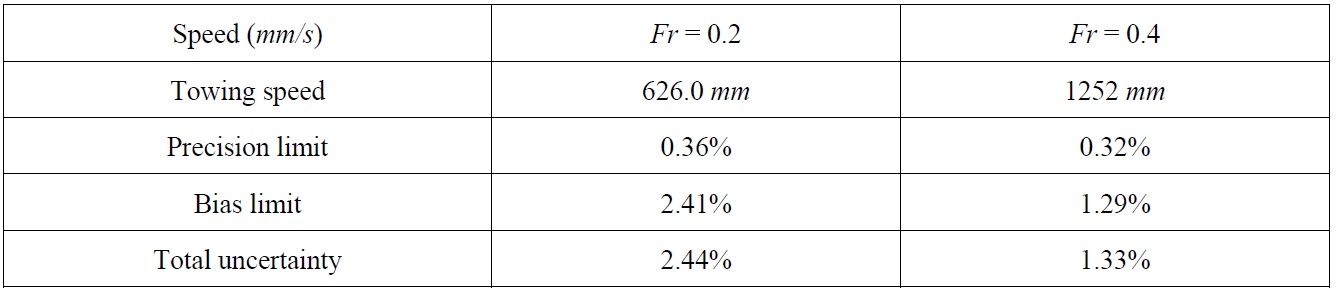
To verify the PIV system, a uniform flow field was measured and compared to the speed encoder signal of the towing carriage. Measurements were conducted at various speeds and depths, as shown in Table 1. A dimensionless variable, u/U, was adopted to compare velocity distributions in different speed conditions.
The non-uniformity of the x-directional component of the velocity was approximately 0.5% of the towing speed. Because of optical characteristics of the camera lens, circular contours were observed, which was considered the primary reason of the nonuniform velocity distribution. Besides the magnitude of the velocity, standard deviation of velocity fields is important to validate the PIV system as it describes the precision error of the experiment. The standard deviation of the x-directional component of the velocity was less than 1% of the towing speed in each case. Through the uniform flow test with 200 particle image pairs, it was estimated that the error level influence of the underwater PIV system on the flow was under 1% of the towing speed, and it is mainly due to the optical limitation of PIV system, not the flow interference of the waterproof casing.
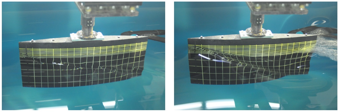
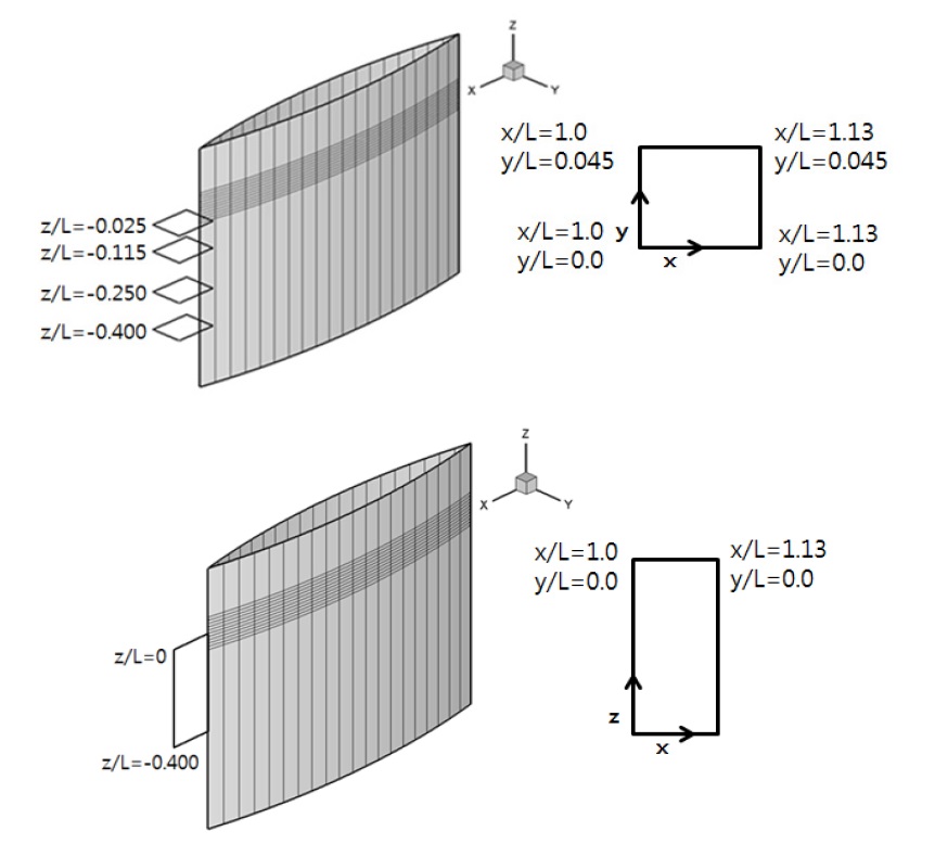
The selected test model was a cylindrical geometry formed by extruding the Wigley hull’s waterplane shape in the vertical direction (see Figs. 2 and 3). The model size was 1 m long, 0.1 m wide and 0.6 m deep from water surface. Flow separation was hardly observed in the flow around this geometry and the free-surface effects could be clearly identified in its turbulent wake. A row of cylindrical type studs were installed at x/L = 0.05 to stimulate the turbulent flow. The surface of model was colored flat black to reduce the reflection of the laser sheet.
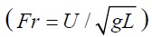
The towing speed of the model was set in terms of Froude number
of 0.2 and 0.4, which represent typical speeds of commercial ships and combatants, respectively. The corresponding Reynolds numbers ( Re = ρUL / μ ) were 5.41 × 10⁵ and 1.08 × 10⁶, respectively. Fig. 2 shows the snapshots of the free-surface flow around the model when it was being towed.
The time interval between two PIV images was set differently for each towing speed, i.e., 2 ms and 1 ms for Fr of 0.2 and 0.4, respectively. During the time intervals, the displacement of a tracer particle was expected to be approximately 20 pixels. However, as the wake flow was slower than the far field flow, the actual displacement was expected to be less than 10 pixels. For each test case, 200 pairs of particle images were captured and averaged into one vector field.
The measurement areas were carefully chosen to identify the free surface wave effects (Fig. 3). Firstly, particle images on the x-z (vertical) planes along the model centerline were captured. As the field of view was limited due to the optical arrangement with the camera position and the focal length of the camera lens, six measurement areas were selected, and the derived vector fields were integrated into a single vector field. The flow fields in x-y (horizontal) planes were captured at the depth of 25 mm (near the free surface), 115 mm, 250 mm (intermediate) and 400 mm (deep enough to be two dimensional).
A cross-correlation method based on the 2D fast Fourier transform with median filtering was used to obtain the velocity vectors. The size of interrogation window was 32 pixels × 32 pixels with 50% overlap. After the correlation process, an average filter was applied to identify error vectors. In addition, a total average of those vector fields was calculated to get the representative vector field of each measurement area. In capturing the images near the free surface, where the shadow of breaking wave and induced bubbles were the primary source of error vectors, a range filtering based on the y-directional velocity component was employed. Lastly, the vector fields were averaged into one vector field. In the averaged vector field, averaged velocity, standard deviation and correlation coefficient of vectors were calculated. For analysis of the flow characteristics, each component of velocity in experimental results was nondimensionalized by the towing speed and each component of Reynolds stress from ensemble-averaged velocity field was divided by square of the towing speed, same as uniform flow measurement.
The uncertainty assessment of the velocity components was conducted following the International Towing Tank Conference (ITTC) standard procedure (2008), which is concerned with the velocity vectors in 2D PIV measurements. In the uncertainty assessment, the measured flow speed by PIV measurements can be written as

where α, magnification factor, is defined as the ratio of physical distance to the pixel length on the particle image from calibration and δu represents the uncertainty from the experiment. Using the ITTC standard procedure, each term from the equation above could be analyzed into uncertainty elements and the bias error limit was calculated. In addition, the precision error limit was calculated using the standard deviation of the distribution of velocity vectors in uniform flow measurements with 200 vector fields. From the precision and bias error limits, the combined uncertainty was evaluated. According to the uncertainty assessment for the reliability of 95%, the combined uncertainty for the velocity components was 2.4% and 1.3% of the towing speed for Fr’s of 0.2 and 0.4, respectively (Table 2). In the experiments, the bias limit was estimated much larger than the precision limit and major source of bias error is the calibration factor, α. The uncertainty assessment results suggest that efforts to decrease the bias limit such as accurate optical arrangement must be imposed if the total uncertainty is required to be reduced.
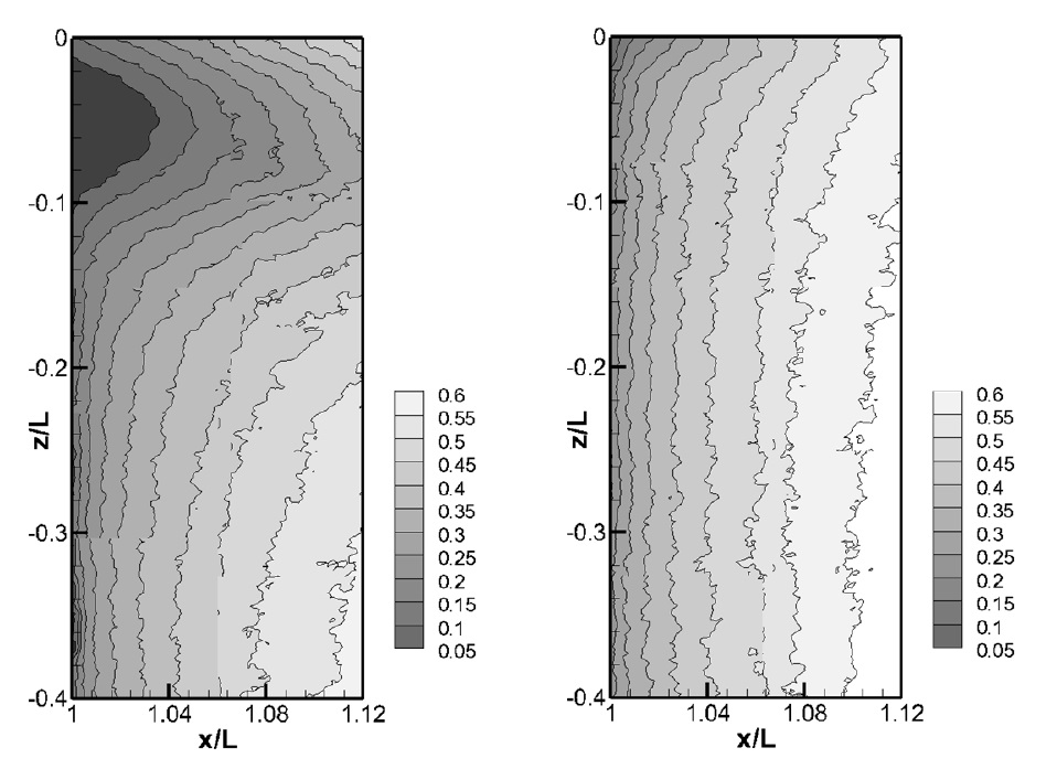
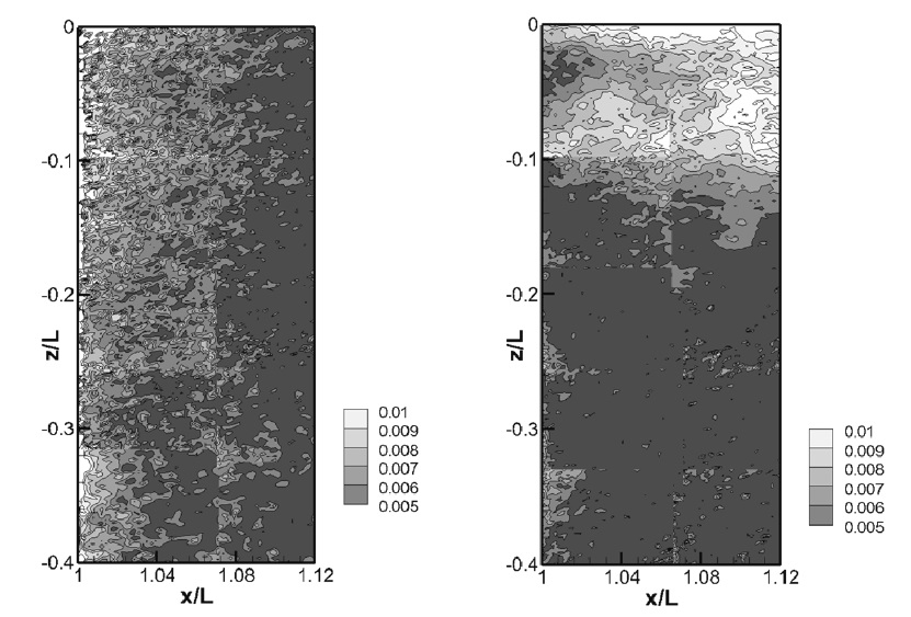
The results are presented in terms of the free-surface effects on the wake pattern and turbulence for two different speeds. Fig. 4 shows the u/U contours in the vertical planes at y/L = 0.0. In all the cases, the free-surface effects, i.e., departure from the 2D wake pattern, were clearly observed near the free-surface. Although the free-surface was not a no-slip wall, it was obvious that its presence had considerable influence on the underlying flow.
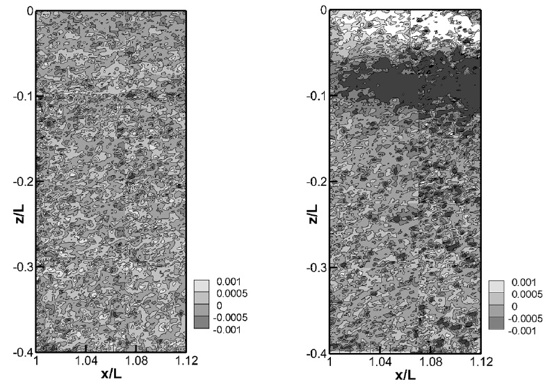
The dimensionless vertical speed, w/U contours in different speeds are shown in Fig. 5. In the measurement at Fr = 0.4, vertical movement is well described near the free surface and two dimensional flow is obviously observed at the deep location.
Another noteworthy was the larger and more significant free-surface effects in the high speed flow case. At Fr = 0.4, the length of the wave generated by the advancing model was comparable to L, and the orbital motion of the water particles at the trailing edge slowed down the wake further than that in the low speed flow case. The influence of the orbital motion was more prominent near the free surface, because the orbital motion attenuates quickly with increasing depth.
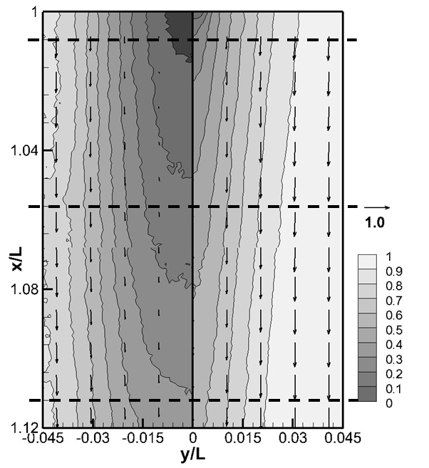
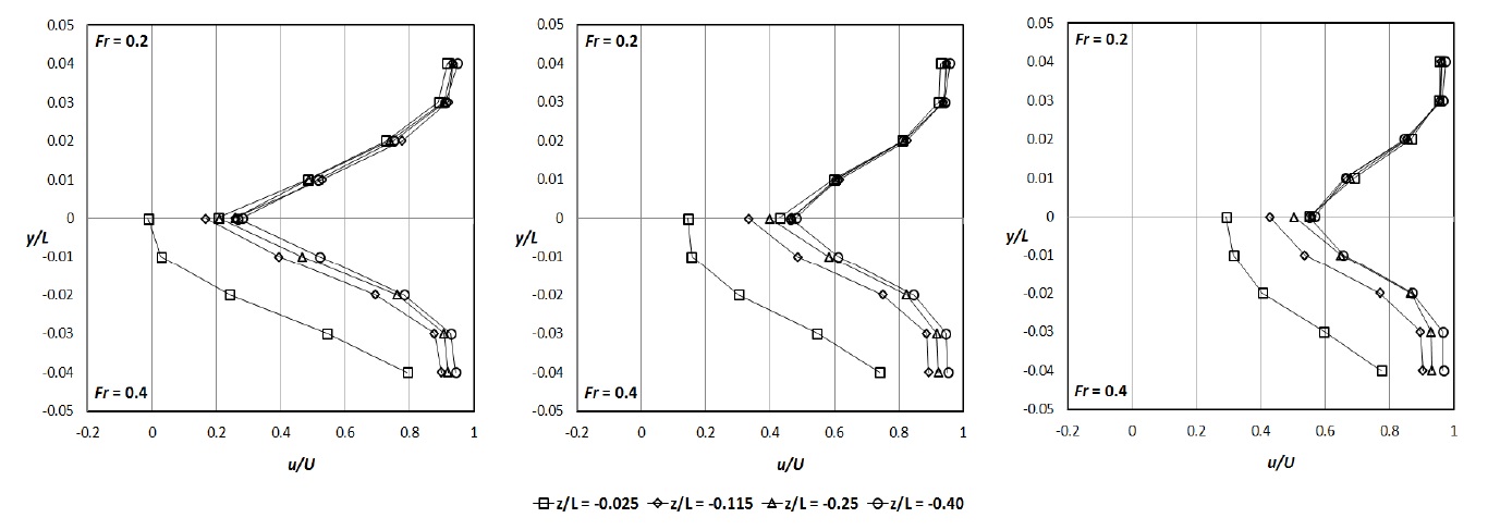
Fig. 6 shows the u/U contours and u-v velocity vectors in the horizontal planes at z/L = -0.025. The measurement at Fr = 0.2 is shown on the right ( 0 ≤ y / L ≤ 0.45 ), while the measurement at Fr = 0.4 is on the left ( ?0.45 ≤ y / L ≤ 0 ). Fig. 7 shows u/U distributions along the dashed lines in Fig. 6 (x/L = 1.01, 1.06, and 1.11) at different depths (z/L = -0.025, -0.115, -0.250, and -0.400). The measurement at z/L = -0.40 was chosen as the reference location for 2D flow. At z/L = -0.025, -0.115, and - 0.25, comparing the measurement at z/L = -0.40, free-surface effects could be identified as the widening of the wake in both the low and high speed flows and the extended wake region due to the free-surface wave, especially in the high speed flows. The latter is also shown as the violent free-surface wake in Fig. 2. Naturally the wake patterns at Fr = 0.2 and Fr = 0.4 flows in the deep location were quite similar, as both were from the fully developed two-dimensional turbulent boundary layer and wake of the test model. Although there was difference in Re, it was not large enough to display significant thinning of the boundary layer and wake.
At Fr = 0.2 and intermediate depths (z/L = -0.115, -0.250), u/U profile converges to that of 2D flow and remains unchanged with increasing depth. Only near the free surface (z/L = -0.025), the recovery of u/U was delayed. At Fr = 0.4, however, the delay of u/U was observed at z/L = -0.115 and -0.250. As also shown in Fig. 4, stagnant flow was observed at z/L = -0.025, which must have affected the velocity field. In addition, since the wave length increased and orbital motion of the water particle was more active at the high speed, the free surface effect, e.g., the delay of the recovery of x-directional velocity, was observed except the 2D flow. Since the 2D velocity data were obtained in PIV measurements, only two components of normal stresses and one shear component could be derived for vertical plane measurements.
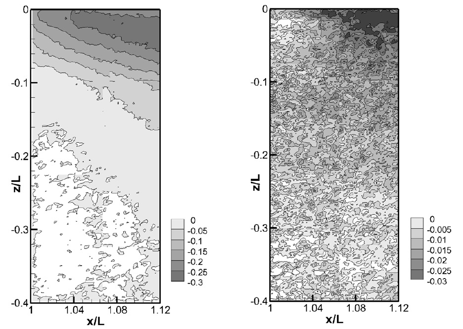
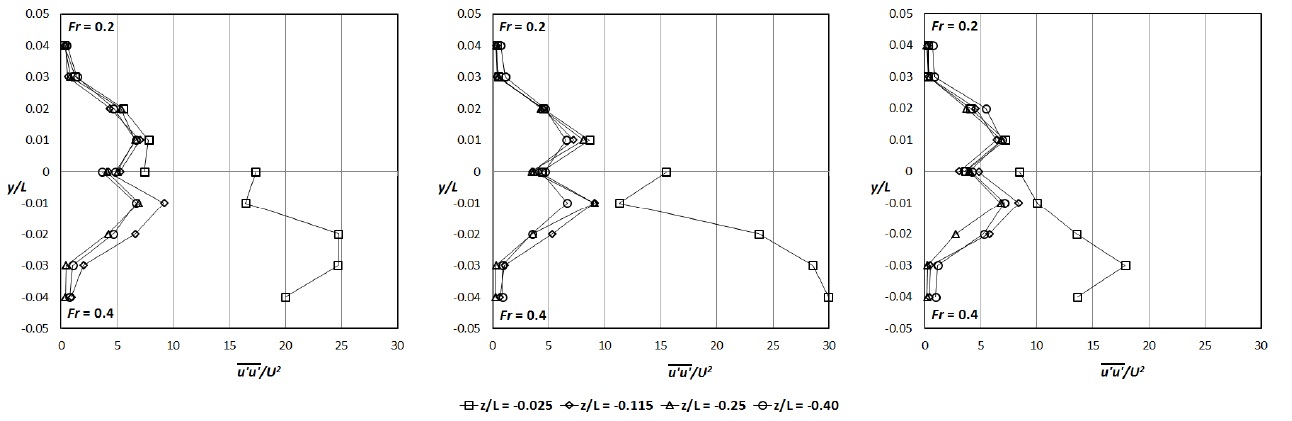
Figs. 8 and 9 show the non-dimensionalized Reynolds normal stresses in the vertical plane. At Fr = 0.2, Reynolds normal stress was just concentrated behind the trailing edge and Reynolds normal stress decreased with the increasing distance. In contrast, the free surface effects on the turbulent wake were clearly identified at Fr = 0.4. With the violent free surface fluctuation, Reynolds normal stress was relatively larger near the free surface than behind the trailing edge. Fig. 10 shows Reynolds shear stress components, at Fr = 0.4, coherent turbulent structure near the free surface was more prominent than the measurement at Fr = 0.2.
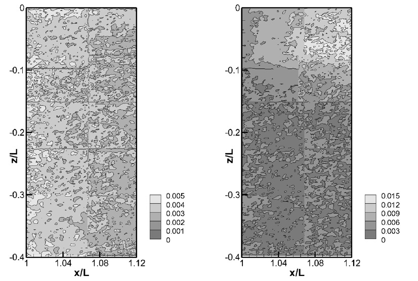
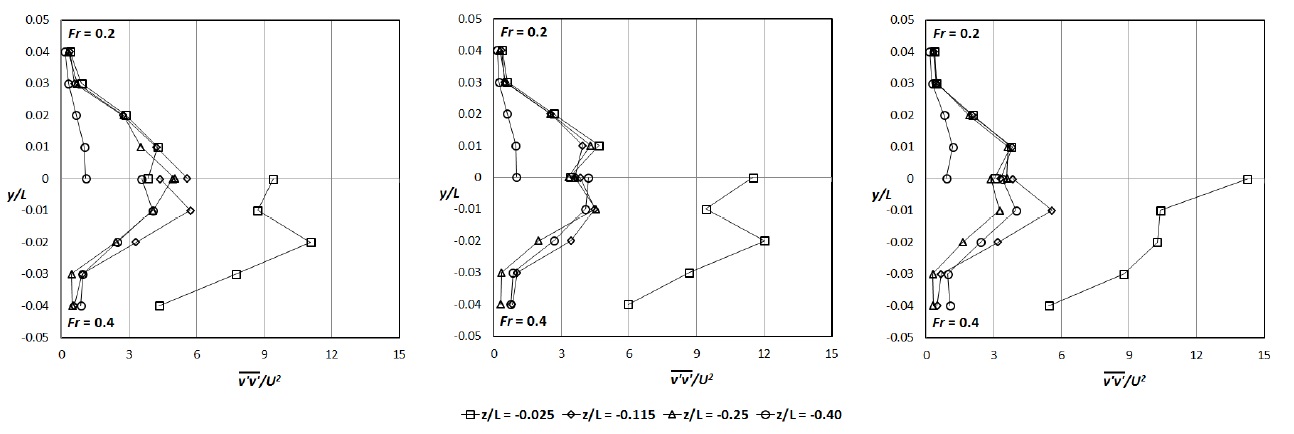
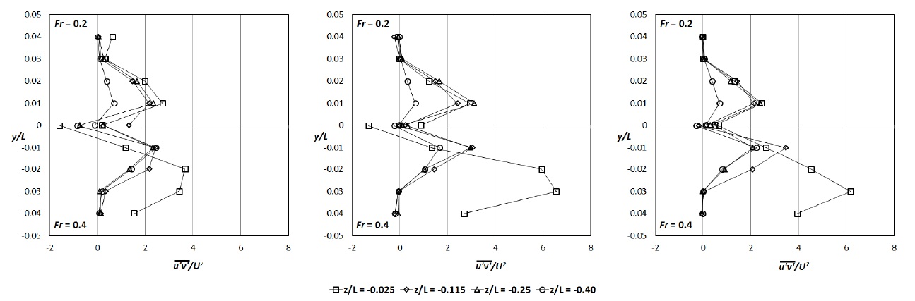
Figs. 11 and 12 show Reynolds normal stress in horizontal planes, like Fig. 6. It is shown that region with strong Reynolds normal stress location coincided with the location of the high velocity gradient. At z/L = -0.025, the difference between two speed conditions was obvious as for the velocity distribution, while no significant difference was identified at z/L = -0.40. Because the violent surface wave was only observed at Fr = 0.4, it seems that the change of the magnitude was strongly affected by the violent free surface. In addition, Reynolds shear stress distributions at the same locations were shown in Fig. 13. In every case, dominant turbulence structure was clearly found where Reynolds shear stress distribution has unique pattern, similar to Reynolds normal stress cases. The magnitude of Reynolds shear stress near free surface was larger than 2D flow at z/L = -0.40, thus it was observed that the free surface flow has significant influences on Reynolds shear stresses as on Reynolds normal stresses.
In this study, the velocity field around a surface piercing body in two advance speeds was measured by a towed underwater 2D PIV system. The uncertainty analysis following the ITTC standard procedure was applied, and the combined uncertainty for the velocity components was quantified as 2.4% and 1.3% of the towing speed for Fr’s of 0.2 and 0.4, respectively.
To identify the free surface effects on the turbulent wake, the flows in the shallow (z/L = -0.025) and deep (z/L = -0.400) locations were compared, and it was observed that the free surface delayed the wake recovery. Also strong interaction between the wake and the free-surface wave behind a surface-piercing body was observed at Fr = 0.4.
Reynolds stresses were utilized to describe the concentration of the turbulence. At Fr = 0.2, higher Reynolds stress was observed behind the trailing edge, while Reynolds stress increased where the velocity changed rapidly at Fr = 0.4.