The movement of underwater vehicles with a suitable combination of body speed and water depth will produce local cavitation on the body. The extent and stability of the vapor cavities so formed may vary from small, discrete, transient bubbles to large and essentially stable bubbles enveloping the rear of the body. When a vapor- or gas-filled cavity grows until it is very long compared with the body dimensions, it is named a supercavity. Supercavities are formed by the growth of a fixed cavity or by the displacement of the liquid in a hydrodynamic wake, either because of a spread of vaporous cavitation, or because of the admission of gas into the low-pressure zones of the wake.
Compressible multiphase flow arises in many natural and industrial situations including bubble dynamics, shock wave interaction with material discontinuities, detonation of high energetic materials, hypervelocity impacts, cavitating flows, combustion systems to name only a few. The motivation of the present study is the accurate and computationally efficient resolution of interface problems in extreme flow conditions, as well as the computation of dynamic appearance of interfaces, that occur in cavitating flows. These interfaces are often separating pure media but also mixtures of materials in which wave dynamics is also important. Godunov type schemes and variants have reached a level of maturity to solve single phase flows in the presence of discontinuities. However, the presence of large discontinuities of thermodynamic variables and equations of state at material interfaces result in numerical instabilities, oscillations and computational failure (Abgrall, 1996; Karni, 1994).
To resolve these difficulties, two classes of methods have been developed. They are Sharp Interface Methods (SIM) and Diffuse Interface Methods (DIM).
In the Lagrangian class of SIM (Hirt et al., 1974; Farhat and Roux, 1991), the computational mesh moves and distorts with the material interface. However, when dealing with fluid flows, deformations are unbounded and resulting mesh distortions can make the Lagrangian approach unpractical (Scheffer and Zukas, 2000). Eulerian methods use a fixed mesh with an additional equation for tracking or reconstructing the material interface. In the volume of fluid (VOF) approach (Hirt and Nichols, 1981) each computational cell is assumed to possibly contain a mixture of both fluids and the volume occupied by each fluid is represented by the volume fraction, transported with the flow. This method is widely used for incompressible flows as there is no special thermodynamics to compute in mixture cells (Gueyffier et al., 1999).
The second type of methods (DIM) considers interfaces as numerically diffused zones, like contact discontinuities in gas dynamics. Diffuse interfaces correspond to artificial mixtures created by numerical diffusion. A pioneering work in this direction was performed by Abgrall (1996). Determination of thermodynamic flow variables in these zones is achieved on the basis of multiphase flow theory (Saurel and Abgrall, 1999; Abgrall and Saurel, 2003; Saurel et al., 2003; Murrone and Guillard, 2005; Abrall and Perrier, 2006; Saurel et al., 2007; Petitpas et al., 2007). The challenge is to derive physically, mathematically, and numerically consistent thermodynamic laws for the artificial mixture. The important issue is to fulfill interface conditions within this artificial mixture.
In this study, transient axisymmetric simulations of cavitating flows are performed using a diffuse interface model. The numerical method was used for cavitators with different geometries in a wide range of cavitation numbers and the results are compared with those of analytical relations.
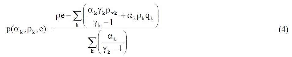
The diffused interface model, proposed in Saurel et al. (2009), is used in the computations of multiphase flow with an arbitrary number of fluids. The model is able to compute interfaces and fluid mixtures evolving under a unique pressure and unique velocity. It is thus particularly well adapted to cavitation studies with dynamic appearances of supercavity. The model is as follows:
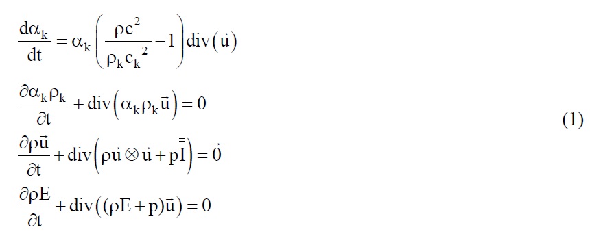
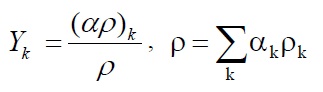
where
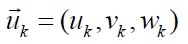
are the volume fraction, the density, the velocity vector of the phase k.
p and
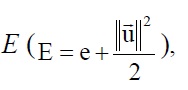
The mixture internal energy is defined as follows:

where
Each fluid is governed by its own convex equation of state (EOS), ek = ek (ρk, p), that allows the determination of the phases’ sound speed, ck = ck (ρk, p). In the particular case of fluids governed by the stiffened gas EOS,

the resulting mixture EOS reads,
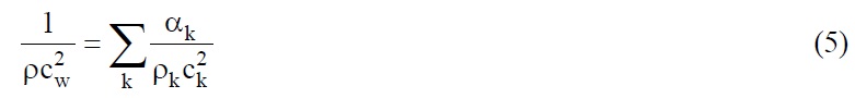
System (1) is hyperbolic with the three wave’s speeds u, u + cw and u?cw where cw is the multiphase extension of the non-monotonic Wood sound speed (Wood, 1930):
System (1) is also thermodynamically consistent as it agrees with the second law of thermodynamics. But system (1) presents inherent difficulties for its numerical solution. The difficulties are as follows:
(1) Volume fraction positivity: How to treat the non-conservative term in the volume fraction equation when shocks or strong rarefaction waves are present?
(2) The volume fraction varies across acoustic waves: Riemann solver is difficult to construct.
(3) The mixture sound speed has a non-monotonic behavior.
A pressure non-equilibrium model is built to circumvent these difficulties (Saurel et al., 2009). It is solved by a 4-step method:
(1) At each cell boundary solve the Riemann problem with the HLLC solver (Toro et al., 1994; Toro, 1997).
(2) The N-phase pressure non-equilibrium flow model is solved without relaxation effects with a Godunov-type scheme.
(3) A pressure relaxation solver is used to reach pressure equilibrium.
(4) Internal energies rest is achieved with the help of the mixture total energy to guarantee shock waves transmission through interfaces and improve robustness.
>
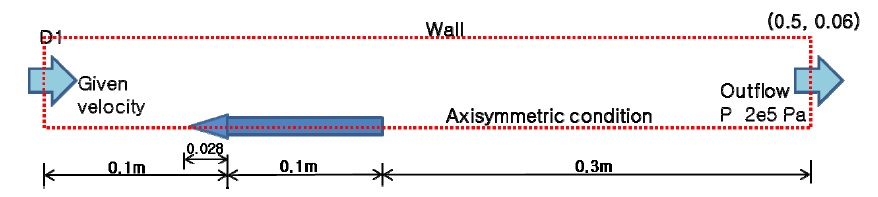
Computational domain and flow conditions
In this study, transient axisymmetric simulations for 2D supercavitating flows shown in Fig. 1 are performed using a diffuse interface model. Calculations for supercavitating flows around various cavitators (30°, 45° cones and disks) were performed. The left boundary of the computational domain is velocity inlet boundary condition with given velocity (20, 25, 30, 40, 50 and 60
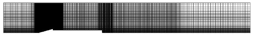
Grids generated by the cartesian grid were concentrated around a head and end of the body, as shown in Fig. 2. The grid consisted of approximately 30,000 cells. Courant-Friedrichs-Lewy condition (CFL) number was set to 0.4. Using Xeon (2.4
When the pressure in a liquid flow falls below the corresponding vapor pressure, the liquid evaporates. This phenomenon, named cavitation, has a crucial effect on the performance of hydraulic systems. Pumps, nozzles, turbine blades, and hydrofoils are just a few examples where the occurrence of cavitation is an important design issue. Cavitation is categorised by a non-dimension number called cavitation number as follows:
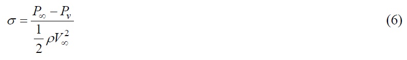
In this,
Shape of supercavity and drag coefficients are important parameters on the study of supercavitating flows. The relations which are indicated as theory are based on Reichardt’s analysis (Reichardt, 1946; Self and Ripken, 1955). The relations are as follows:

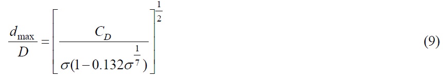

In these,
Disk drag coefficient by the approximate theory of Pleseet and Shaffer can be represented for σ up to 1.5 by an interpolation formula as follows:

This result was obtained by rotating the two-dimensional flat-plate pressure distribution about the axis of symmetry.
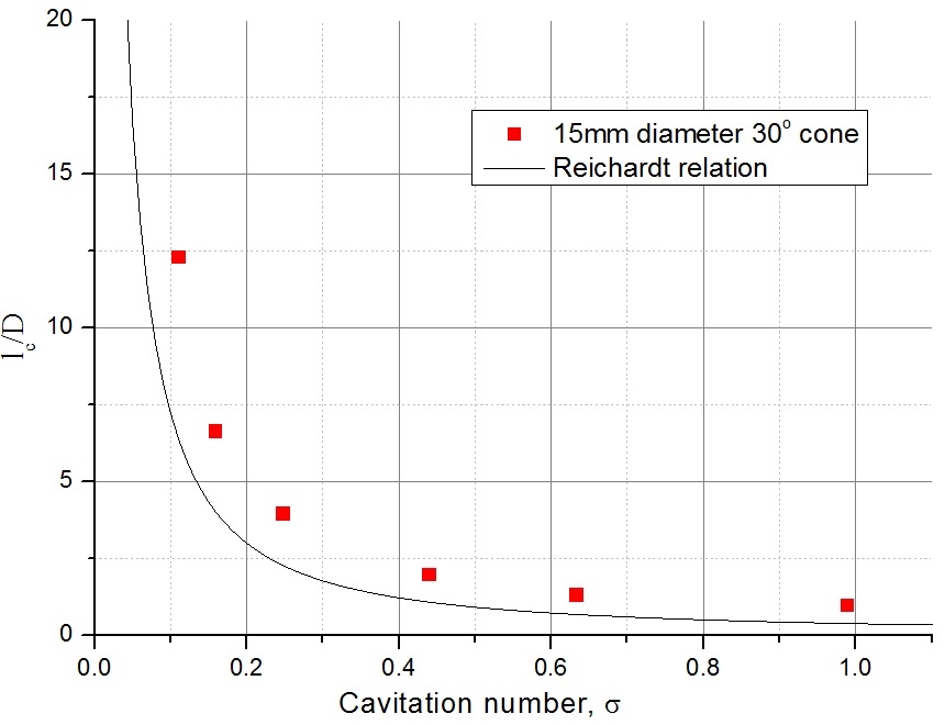
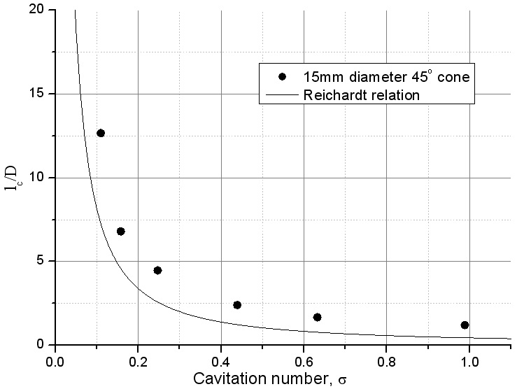
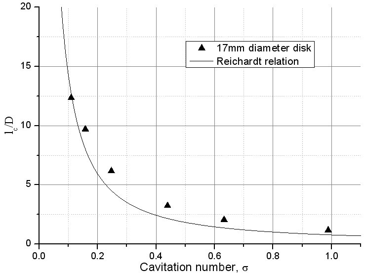
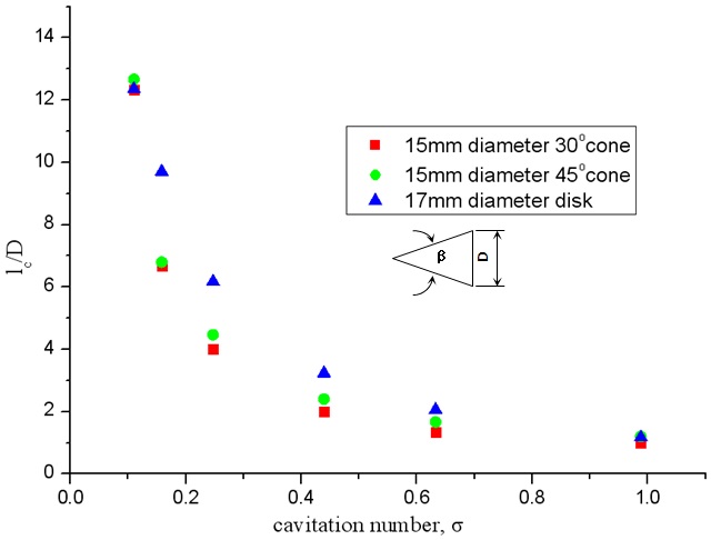
The cavity dimensions obtained from numerical results for 30°, 45° cones and disks are shown in Fig. 3. It is notable that for cavitation numbers above approximately 0.44, the cavitators with larger angle β tended to produce larger cavities. Decreasing σ results in an increase in the length of the supercavity, with the dramatic increase in low cavitation number.
In Figs. 4 to 6, the computed results were compared with analytical relations. It can be seen that the numerical results compare well with analytical relations. In low cavitation number, the discrepancy between the relations and numerical results may be attributed due to the effects of the wall. According to Franc and Michel (2004), in a flow confined by solid walls, the cavity becomes infinite for a value of the cavity pressure
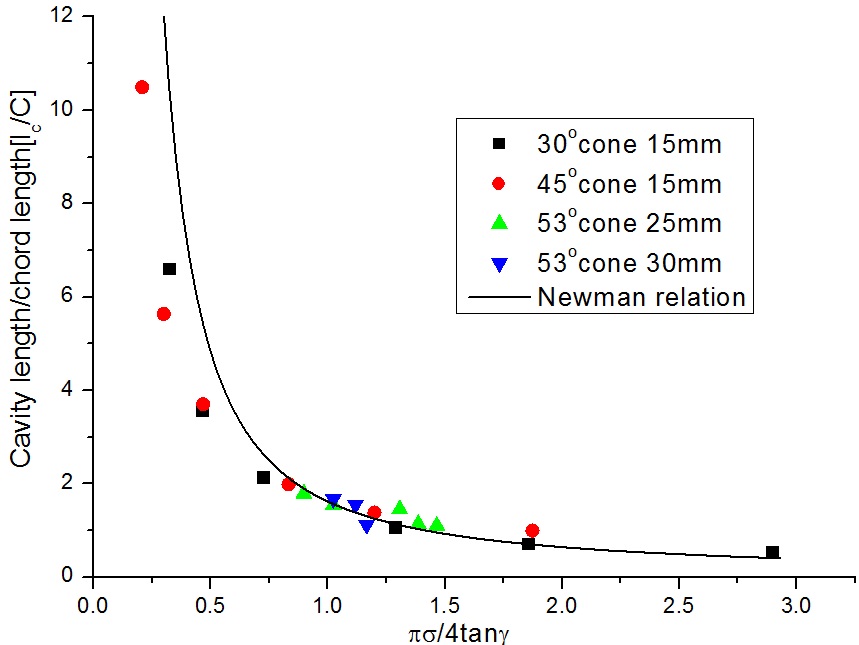
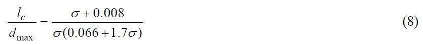
Also, predicted cavity length was compared with an analytic solution derived by Newman (1977) in Fig. 6. The relation shows the relationship between the cavitation number (σ) and the cavity length (
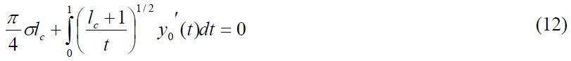
where
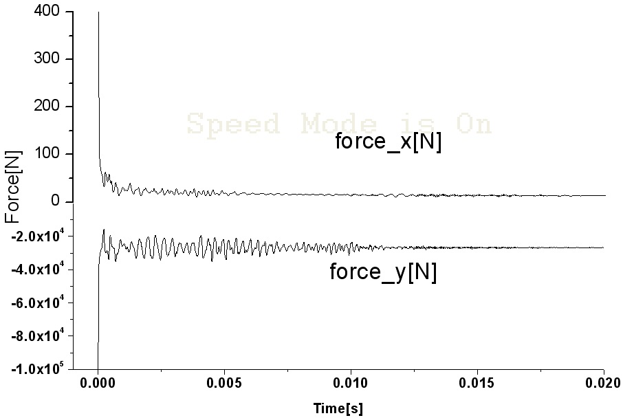
The evolution of the resulting pressure force on the cavitator is shown in the Fig. 8. During the first times, the force is very big as results of initial conditions stiffness that produce a shock wave. When the flow reaches quasi steady state, it is convergence.
Drag coefficient for each cavitor was obtained when considering the definition as shown below:
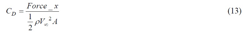
where A = (1/4)πD2.
The drag coefficient against cavitation number is plotted in Fig. 9. As shown in the figure, a good agreement is observed between the results of the model with analytical relations. Important point is that as cavitation number decreases, in other words velocity increases, the drag coefficient decreases.
Diffuse interface model for numerical analysis was used to predict the cavitation that occurs behind axisymmetric cavitator in a liquid flow. The computed results were compared with relation by Reichardt. Drag coefficient obtained from pressure forces acting on the cavitator also compared well with those obtained from analytical relations. The size of cavity is associated with a certain head form. Decreasing cavitation number yields an increase in the length of the supercavity, with the dramatic increase in low cavitation number.