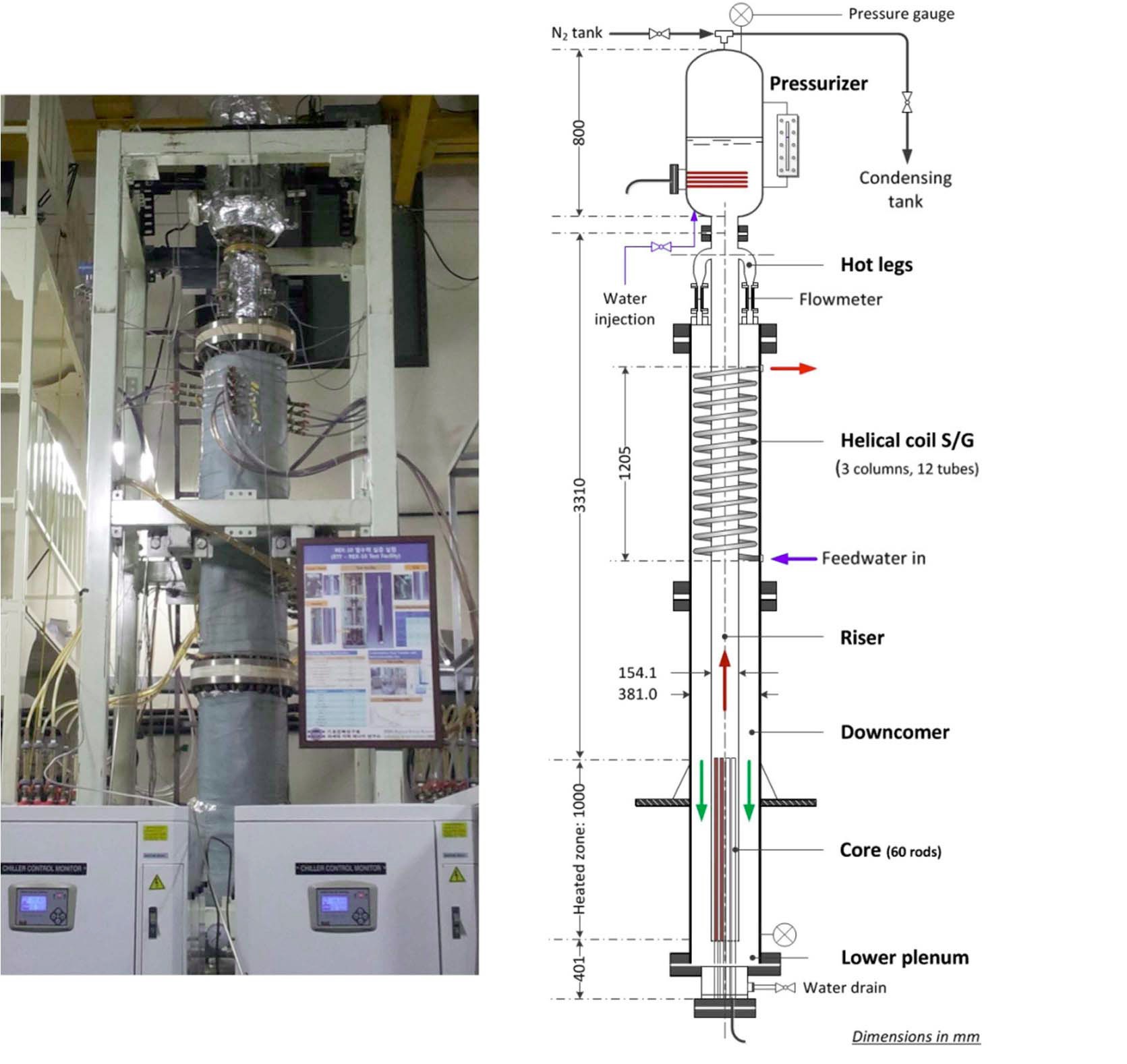
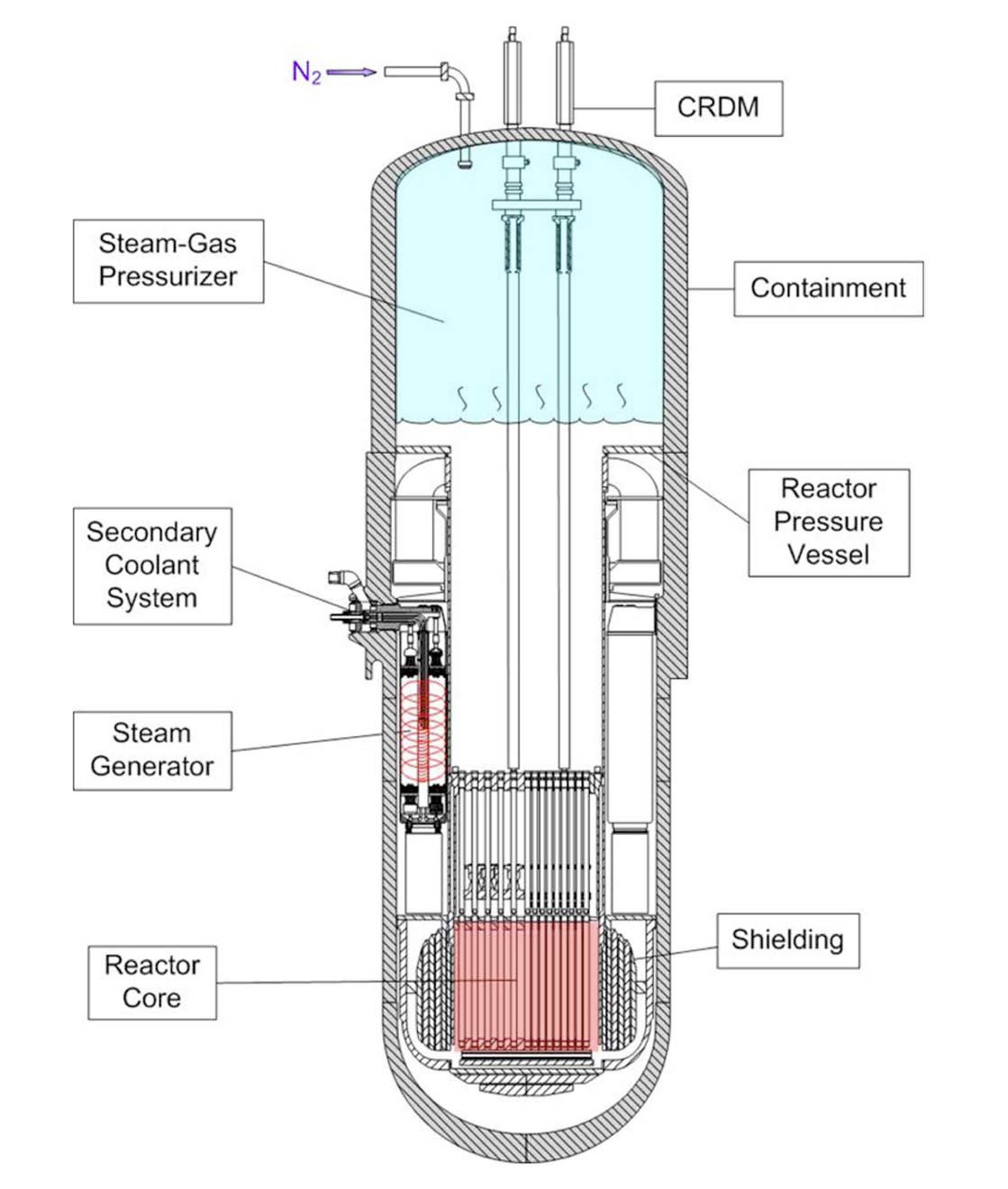
The passive safety features of nuclear reactors have emerged as a central issue in both industry and academia in the aftermath of the Fukushima nuclear disaster, resulting from a prolonged power outage. Development of passive safety systems such as PRHRS [1], PAFS [2], and PCCS [3] is an effort to incorporate passive safety into PWRs, and the implications from the accident have been deliberately reflected in the recent design of advanced small modular reactors (SMRs) as well. Among a variety of SMRs being developed around the globe, REX-10 [4] may accommodate the highest level of passive features in operation and mitigation of accidents. REX-10 was designed by Seoul National University (SNU) to provide small-scale electricity generation and nuclear district heating. It is a fully-passive integral PWR in which the coolant flow is driven by natural circulation, the system pressure is regulated by a built-in pressurizer with non-condensable gas, and the decay heat is removed by the actuation of PRHRS after reactor shutdown. The schematic diagram of REX-10 is shown in Fig. 1.
In describing the thermal-hydraulic behavior of a fullypassive integral PWR such as REX-10, one may use commercial system codes such as RELAP5 [5], RETRAN-3D [6], and CATHARE [7], which have reached a high degree of maturity through extensive qualifications. However, these generic codes do not always incorporate the mathematical models for reactor components of integral PWRs. In practice, the RELAP5 and RETRAN-3D do not contain thermal-hydraulic models of a helical-coil steam generator (S/G) and an in-vessel pressurizer with a non-condensable gas, respectively. In addition, it is not easy for a user to modify and supplement the required physical models in the source codes on account of their complex structures.
In the transient simulation and the safety analysis of an integral PWR, one of the major computational challenges is associated with the mathematical modeling needed to present an innovative reactor component [8]. Since the nuclear societies have focused on numerical studies of thermal-hydraulics in a loop-type large-scale NPP, a system analysis code specifically for an integral reactor is rarely found. One exception is the TASS/SMR code developed by the Korea Atomic Energy Research Institute. TASS/SMR is a system code to simulate all relevant thermal-hydraulic phenomena in the RCS of SMART during operational transient and design basis accidents [9]. In order to simulate the design characteristics of SMART, TASS/SMR incorporates specific heat transfer models such as the helical-coil S/G model and the condensate heat exchanger model in the PRHRS. However, since the field equations of TASS/SMR are based on the homogeneous equilibrium model (HEM), there might be some restrictions on some transients in which the non-equilibrium effects are dominant.
To assess the design decisions and investigate the transient RCS behavior of a fully-passive integral PWR such as REX-10, a thermal-hydraulic system code named TAPINS is developed at SNU. TAPINS can be defined as an in-house code for particular application to a specific type of nuclear reactor, rather than a generic code developed in a systematic way to cover a wide range of nuclear systems. Current TAPINS has been improved from the previous version [4] based on the momentum integral model, which consists of simple governing equations formulated from the HEM, by employing a more sophisticated two-phase flow model and numerical solver. TAPINS is characterized by applicability to transients with non-equilibrium effects, better prediction of the transient behavior of a pressurizer containing non-condensable gas, and code assessment by using experimental data from the autonomous integral effect tests in the RTF (REX-10 Test Facility).
The code structure, thermal-hydraulic models, and input module of TAPINS are specialized for an integral PWR. Several essential modules to describe the RCS of an integral PWR, such as the heat conduction module of fuel rods in the core and helical tubes in the S/G, are hardwired in component models of TAPINS. Compared to the generic system codes, more convenient pre-process is possible with a minimized number of input data fields under the frame which divides the RCS of an integral PWR into six subsections [4].
TAPINS adopts a one-dimensional four-equation driftflux model (DFM) as field equations. It also consists of component models for the core, the once-through helicalcoil S/G, and the built-in steam-gas pressurizer. In particular, a dynamic model to estimate the transient responses of the pressurizer containing the non-condensable gas is newly proposed and incorporated into TAPINS. In addition, TAPINS includes proper heat transfer coefficient correlations and the heat conduction model to predict the timedependent heat transport in the core and the helical-coil S/G of a fully-passive integral PWR. The discretized governing equations through the semi-implicit scheme on the staggered mesh are solved by the Newton Block Gauss Seidel (NBGS) method.
This paper presents an overview of the TAPINS hydrodynamic model. TAPINS has been verified and validated with 7 sets of assessment problems ranging from fundamental benchmarks to the IET performed in a scaleddown apparatus of REX-10 [10]. Among these V&V results, a selection of simulations that reveals the distinguishing features of TAPINS are introduced in this paper: analyses on the subcooled boiling test, the pressurizer insurge test in the presence of non-condensable gas, and the change in core power test as well as the LOFW (loss-of-feedwater) test in the RTF. The details of the hydrodynamic model and the numerical solution scheme are described in Sections 2 and 3, respectively. In Section 4, the code applications to three assessment problems are presented.
2. HYDRODYNAMIC MODELS OF TAPINS
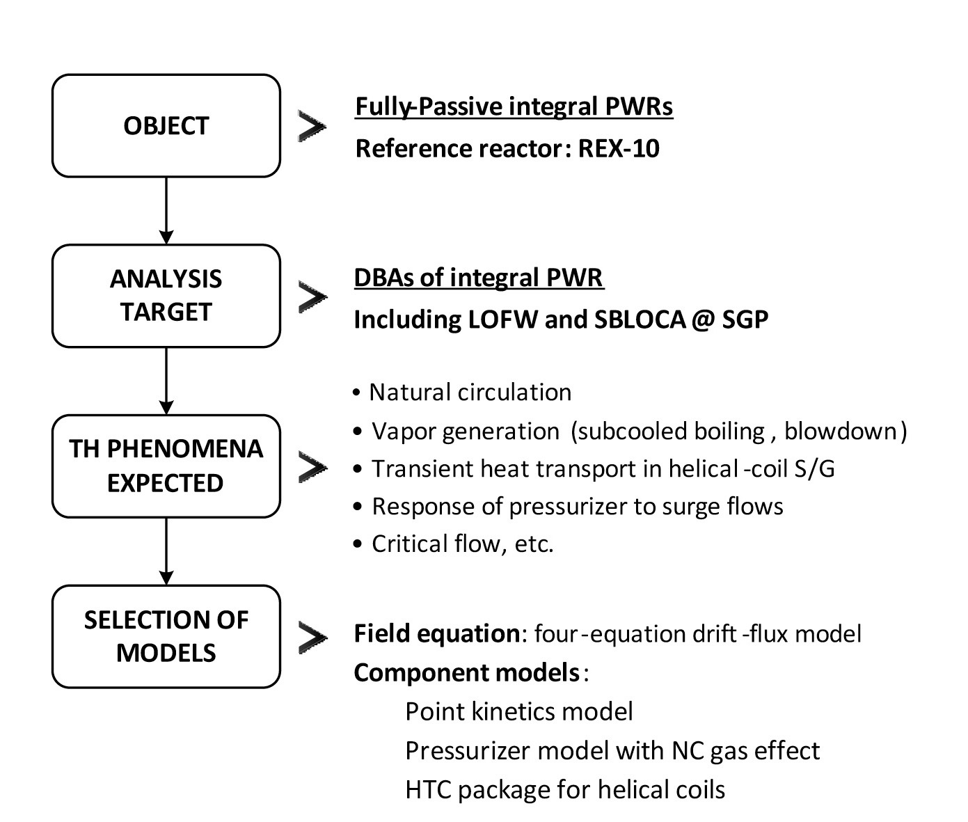
When developing a thermal-hydraulic analysis code, one has to design the fundamental concept and frame of the code prior to programming the software. Then, the specifications as well as the proper models and correlations needed for the analysis code can be determined. As mentioned before, the analysis target of this research is a fullypassive integral PWR in which the reactor is normally operated in a passive manner and accidents are mitigated passively as well. Figure 2 describes the procedure to design the fundamental frame of TAPINS.
The reference reactor typifying fully-passive integral PWRs is set to REX-10 in this study. The reactor transients of interest encompass not only those caused by changes in core power or the variation of the heat transport in the helical-coil S/G, but also the design basis accidents (DBAs) of integral PWRs. By design, an integral reactor can eliminate the possibility of a LBLOCA arising from the rupture of a large pipeline penetrating through the RPV. However, a loss-of-feedwater accident in which the heat removal by the secondary system totally vanishes is a feasible event to threaten the safety of an integral PWR. In addition, a break occurring at the small pipeline connected to the pressurizer vessel, such as the nitrogen injection line, may result in the hypothetical discharge of coolant and system depressurization [11]. Accordingly, this study intends to develop a system analysis code that has predictive capability for the LOFW and SBLOCA of an integral PWR. The thermalhydraulic phenomena expected in these DBAs include natural circulation, vapor generation caused by subcooled boiling or blowdown, transient heat transport in the helicalcoil S/G, pressure response of the steam-gas pressurizer to surge flow, choked flow, and so on.
In selecting the hydrodynamic model, the principle is that one should choose the least complicated model which accommodates the phenomena of interest [12]. Unlike conventional NPPs where long horizontal pipelines are located outside the RPV, the primary circuit of an integral PWR mostly consists of vertically-oriented channels. Thus,
the drift-flux model is selected for the field equations of TAPINS since it can take into account the non-equilibrium effect of two-phase flow phenomena and provide highly accurate predictions for a vertical channel, especially in bubbly and slug flow regimes. Then the constitutive relations associated with relative velocity, interfacial mass transfer, wall friction, and wall heat source have to be supplemented for closure.
For thermal-hydraulic analyses of a fully-passive integral PWR, the mathematical models for major system components typified by the core, the steam-gas pressurizer, and the helical-coil S/G are also needed. Since the multi-dimensional power profile is not essential, the point kinetics model seems to be appropriate in calculating the time-dependent core power in conjunction with the convective heat transport into the coolant. In order to predict the effect of non-condensable gas on the pressure response of an integral PWR, a dynamic model for the steam-gas pressurizer is also required. In addition, the heat transfer package for the shellside and the tube-side of helical tubes according to the boiling region has to be essentially employed.
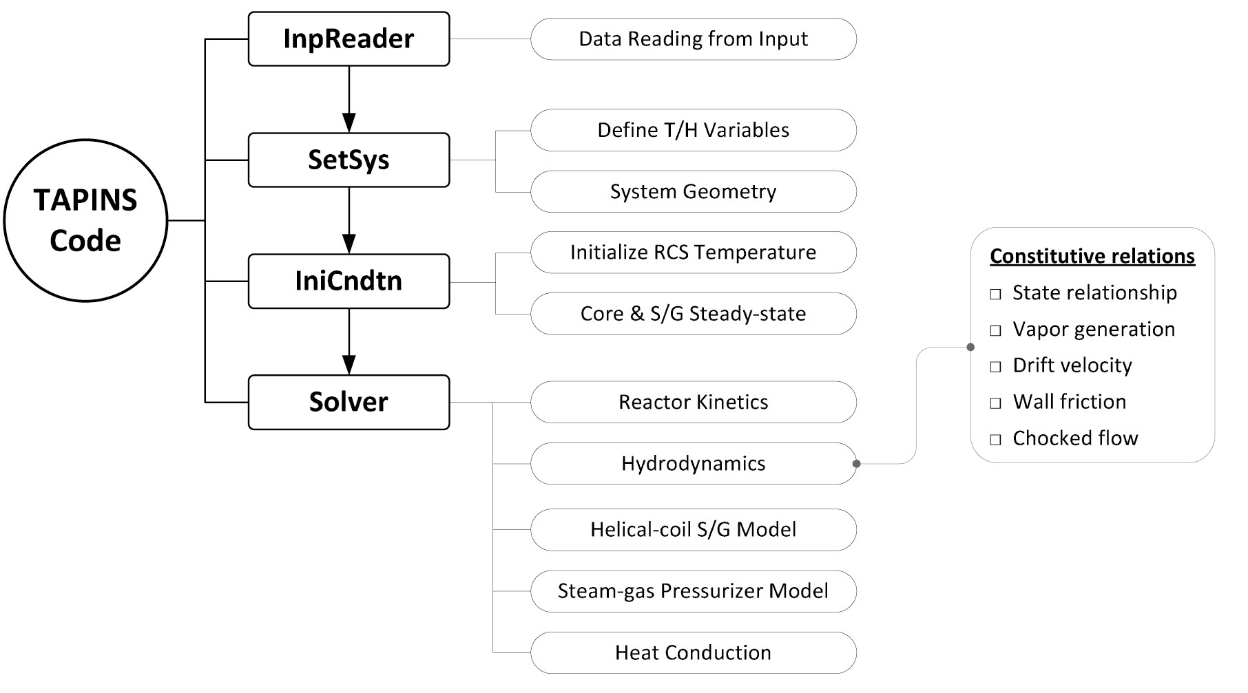
Drawn from the above considerations, the code structure of TAPINS is depicted in Fig. 3. It consists of a couple of large blocks divided by the function in the calculations. TAPINS is written in FORTRAN 90 and easily executed on a PC.
The previous and new versions of TAPINS use the same component models. However, due to the characteristics of the momentum integral model, the previous version has a drawback that its application is restricted only to the simulation of a closed loop. The current TAPINS is designed to have an improved code capability in view of system modeling; the generality is expanded so that flow or pressure boundary conditions are readily implemented for an open circuit. In addition, it can provide more realistic simulation of two-phase flows than the HEM based version.
The TAPINS hydrodynamic model is a one-dimensional four-equation drift-flux model. In the drift-flux model, the dynamics of a two-phase mixture is expressed in terms of the mixture momentum conservation instead of adopting separate balance equations for each phase [13]. The relative motion between the phases is taken into account by a kinematic constitutive equation. Therefore, one can greatly reduce the difficulties commonly encountered when employing a two-fluid model such as mathematical complication and numerical instability caused by interfacial interaction terms. The four-equation drift-flux model is properly applicable to a wide range of thermal-hydraulic phenomena in an integral PWR.
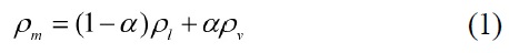
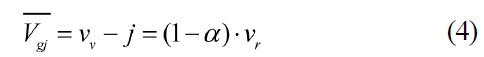
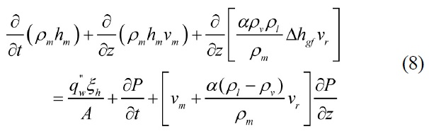
The four-equation drift-flux field equations for a twophase mixture are comprised of two mass conservation equations, one momentum conservation equation, and one enthalpy energy equation. The one-dimensional model is obtained by integrating the three-dimensional model over a cross sectional area and then introducing proper mean values [14]. The average mixture density is given by:
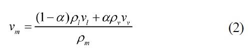
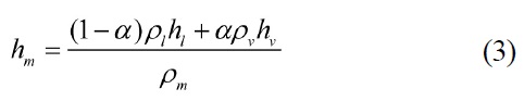
Then, the mixture velocity and the mean mixture enthalpy are weighted by the density as:
The vapor drift velocity is defined as the velocity of the dispersed phase with respect to the volume center of the mixture:
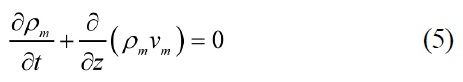
TAPINS utilizes the following forms of four partial differential equations:
Mixture continuity equation
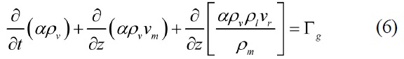
Vapor mass conservation equation
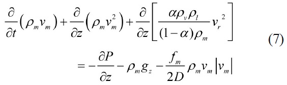
Mixture momentum equation
Mixture enthalpy-energy equation
In the above field equations, the covariance terms, the normal components of the stress tensor in the axial direction, and the mixture-energy dissipation terms are not included since they are negligible. Note that this model accommodates the non-equilibrium effect of two-phase flow by incorporating the mass conservation equation for the vapor, which accounts for the rate of phase change. The vapor generation rate due to phase change is expressed as [15]:
In TAPINS, the vapor phase is assumed saturated; this thermal constraint is regarded as more realistic than the thermal equilibrium between the phases. In addition, the effects of the mass, momentum, and energy diffusion associated with the relative motion between the phases appear explicitly in terms of the drift velocity. In what follows, the constitutive relations needed for mathematical closure of the governing equations are described.
2.3.1 State Relationships
To make a mathematically complete set with the four field equations and the constitutive relations, the equations of state for each phase are needed. The phasic density, temperature, and other saturation properties are called from the steam table [16] in terms of the pressure and the enthalpy energy as:
In the numerical scheme employed in TAPINS, all unknowns appearing in the difference equations, except for the primitive variables, are expressed as functions of the independent state variables. For the linearized definition of those unknowns, several state derivatives are needed in the numerical scheme. All the desired first derivatives of the thermodynamic properties are derived from Bridgman’s table [17] in terms of the isobaric specific heat, the volumetric coefficient of expansion, and the isothermal compressibility. The derivative of saturation temperature with respect to pressure is calculated by the Clasius-Clapeyron equation. The partial derivatives for vapor, which is in saturated state, are obtained by linear interpolation near the saturation value.
While the vapor phase is assumed saturated, the liquid can be either subcooled or superheated. The temperature of metastable liquid is obtained by using a Taylor series expansion about the saturation point as:
The above formulation is derived from a constant pressure extrapolation. On the contrary, for a specific volume of the superheated liquid, the extrapolation along a constant temperature line is employed on account of the inaccuracies that had been reported in some specific cases when using the constant pressure extrapolation [10].
2.3.2 Interphase Heat and Mass Transfer
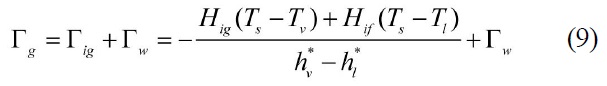
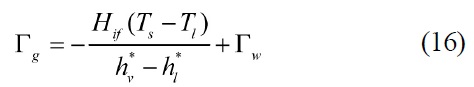
The thermal non-equilibrium effects of a two-phase mixture are accommodated in the drift-flux model by a constitutive equation for phase change that specifies the rate of mass transfer per unit volume. The vapor generation term appearing in the RHS of Eq. (9) consists of the mass transfer due to the interface energy exchange in the bulk and the mass transfer by heat transfer in the thermal boundary layer near the wall. Since the vapor is assumed saturated, Eq. (9) is reduced to:
Here, the terms in the denominator are as follows:
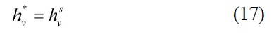
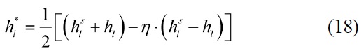
where
η=1 for Гig≥0
= -1 for Гig?0
Thus, the interphase heat transfer coefficient and the mass transfer rate per unit volume near a wall are needed to calculate the rate of vapor generation. Since the interphase heat transfer coefficient depends on the two-phase flow regime, the proper flow regime map has to be incorporated into the code. In TAPINS, both the vertical and horizontal volume flow regime maps are implemented in the same way as RELAP5. In addition, the interphase heat transfer correlations for liquid employed in RELAP5 are adopted in TAPINS. The code calculates the interfacial heat transfer coefficient for the bulk fluid according to the state of the liquid (subcooled or superheated) and the two-phase flow regime. Note that to prevent discontinuity or sharp changes of the interphase heat transfer coefficient, a couple of smoothing techniques are incorporated in TAPINS for under-relaxation.
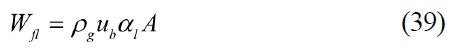
The mass transfer rate per unit volume near a wall is calculated by the Lahey method [18] as follows:
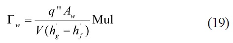
The multiplier denotes the fraction of the boiling heat flux which causes steam generation. It is defined as:
where
The rate of phase change near a wall is calculated only when a positive (boiling) or negative (condensation) heat flux exists.
2.3.3 Wall Friction
In TAPINS, the Darcy friction factor is computed from correlations for laminar and turbulent flows with interpolation in the transition regime. When the Reynolds number is less than 2200, the laminar friction factor is calculated by the theoretical relation,
2.3.4 Drift Velocity
In the drift-flux model, as stated above, the dynamics of the two-phase flow is formulated in terms of the mixture center-of-mass velocity (
In TAPINS, the Chexal-Lellouche model [22,23] is used as a kinematic constitutive equation to predict the drift velocity. The Chexal-Lellouche slip model is applicable for a much wider range of conditions and more detailed in its representation than any other correlations. The model eliminates the need to know the two-phase flow regime. In addition, it has been validated against the vast amount of data to cover the co-current or counter-current flows in vertical and horizontal channels. From the Chexal-Lellouche model, not only the distribution parameter (
The distribution parameter is expressed as:
The drift velocity, to account for the vapor velocity with respect to the volume center of the mixture, is given by:
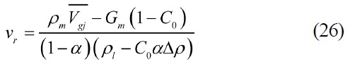
The details of the parameters appearing in Eqs. (22) and (23) are found in the publication of Chexal and Lellouche. From the drift-flux relationships, each phasic velocity can be obtained by:
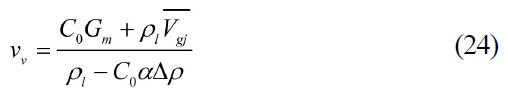
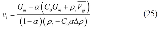
Thus, the relative velocity is:
2.4.1 Point Reactor Kinetics
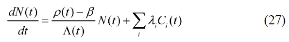
To determine the time-dependent behavior of the fission power, point kinetics equations with six delayed neutron groups are solved in TAPINS. By allowing the spatial dependence to be eliminated, the point reactor kinetics yields solutions for the neutron population density and delayed neutron precursor concentrations from this set of coupled ordinary differential equations:
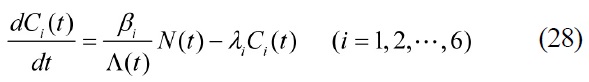
The change in the reactivity induced by the negative feedback effect is also taken into account. The reactivity feedbacks caused by the variation of the core-averaged fuel element and the coolant temperatures as well as the externally introduced reactivity are of great importance:

The neutron kinetics parameters and the reactivity temperature
[Table 1.] Core Heat Transfer Coefficient Correlations in TAPINS
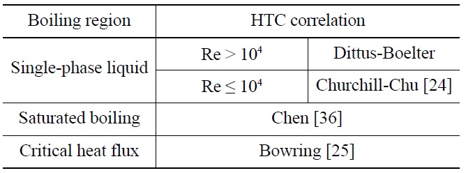
Core Heat Transfer Coefficient Correlations in TAPINS
coefficients are given in the input data of the TAPINS model.
The heat conduction equation is also solved in cylindrical coordinates so that the radial temperature distribution in the fuel rods is determined. With the axial heat conduction neglected, the transient heat transport in fuel elements is represented by a model of a typical fuel rod to obtain the average fuel temperature and the cladding surface temperature. The temperature dependence of the thermal conductivity is explicitly modeled. The boundary conditions for the fuel-cladding gap and the cladding-coolant interface are implemented by supposing a quadratic temperature profile in the vicinity of the boundaries and imposing heat flux continuity.
The core heat transfer coefficient correlations incorporated in TAPINS are summarized in Table 1. By this time, the heat transfer models of TAPINS are prepared for up to the DNB point. To obtain the convective heat transfer rate into the coolant, a correlation suggested by Churchill and Chu [24], which is suitable for free convection flows, is used as a default model for the single-phase liquid. For turbulent flow in the range of
2.4.2 Steam-gas Pressurizer Model
As a unique contribution of this study, a dynamic model of the steam-gas pressurizer is proposed and incorporated into TAPINS for better prediction of the transient response of the pressurizer in the presence of non-condensable gas. Located at the upper head region of the RPV, the steamgas pressurizer is equipped with no active system; instead of controlling a heater or spray, it pursues the passive operation of an integral PWR by containing a certain amount of non-condensable gas such as nitrogen in the gaseous mixture.
Several investigators have proposed pressurizer models, ranging from the two-region model [26] to the three-region non-equilibrium model [27]. However, the previous models deal with a pressurizer containing only steam in the upper gas region and thus the presence of the non-condensable gas is not coupled with the pressure behavior. Since the non-condensable gas affects not only the intensity of mass diffusions occurring in the pressurizer but also the total pressure responses to the transients, a new model accounting for the effect of non-condensable gas is indispensable.
In order to analyze the thermal-hydraulic characteristics of the steam-gas pressurizer, Kim et al. [28] proposed a two-region non-equilibrium concept by extending the RETRAN/3D-INT model. Kim [29] also developed a tworegion model which includes various local mass transfer models in the presence of non-condensable gas and applied it to his own experiments.
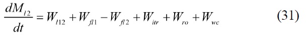
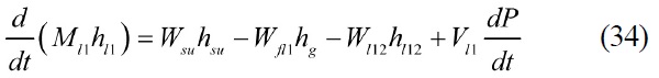
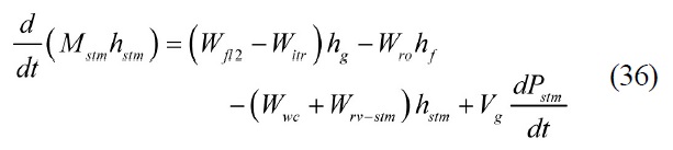
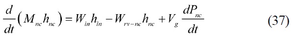
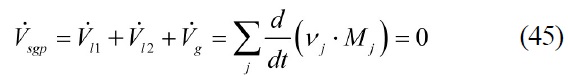
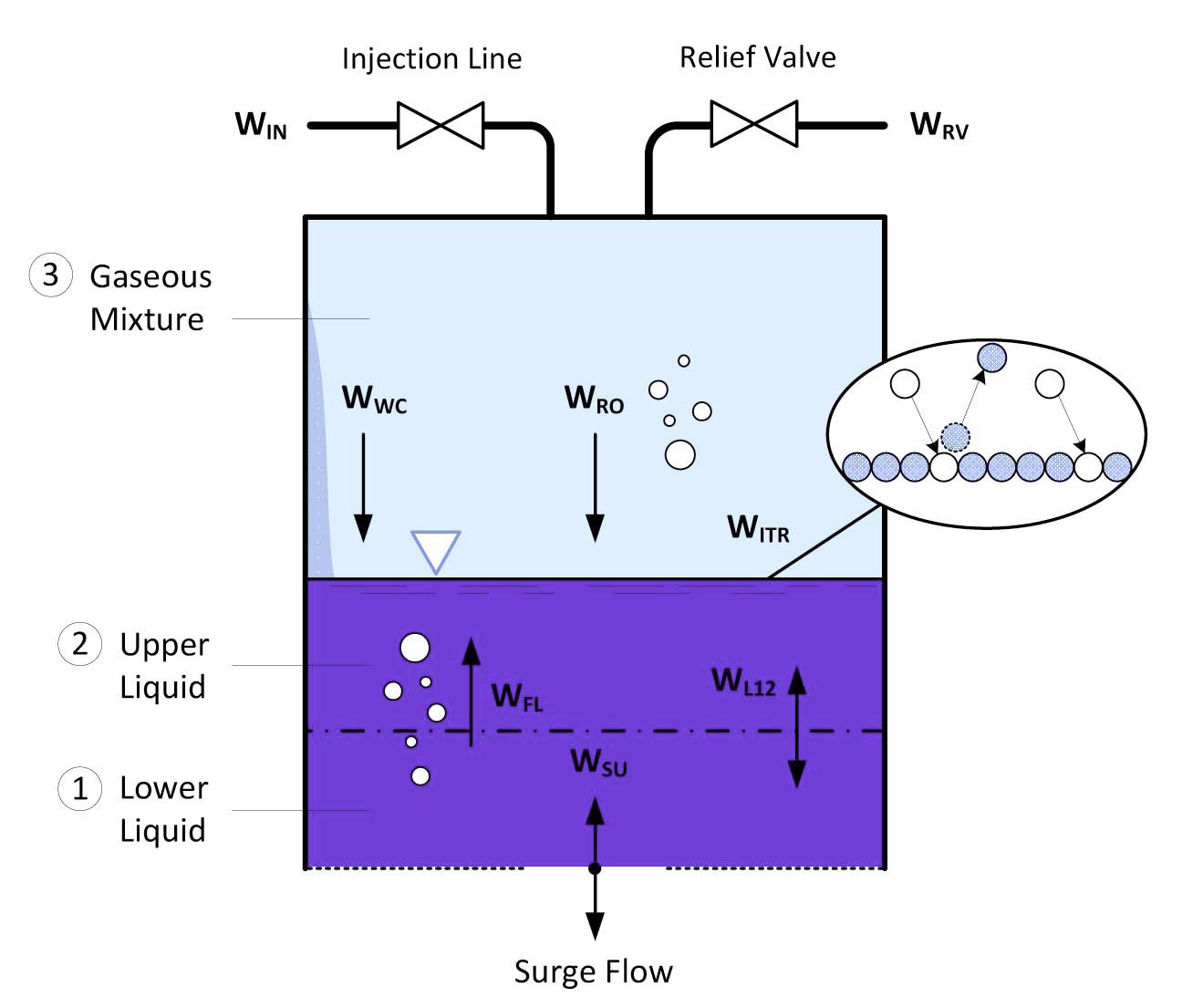
The steam-gas pressurizer model of TAPINS is a threeregion non-equilibrium model based on the basic conservation principles of mass and energy. The pressurizer volume is separated into three distinct regions, each establishing its own thermodynamic state: the gaseous mixture, the upper liquid region, and the lower liquid region. By thermal stratification, the lower liquid region is immediately influenced by surge flow while the floating hot liquid layer in the upper region stays with little change in temperature. Thus, the height of the lower liquid region should be equal to (or greater than) the penetration depth of an insurge flow so that the boundary between the liquid regions can specify the mixing region. Based on a couple of assumptions [10], the model takes into account all the processes of heat and mass transfer that occur inside the pressurizer volume as well as the surge flow from the primary loop. The conservation equations are applied to the steam, non-condensable gas, and two regions of liquid water. Physical phenomena to be modeled include surge (
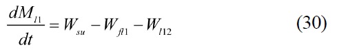
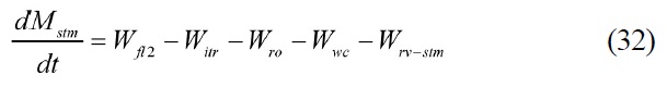
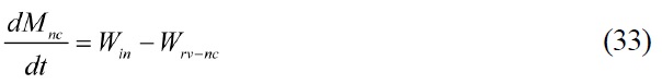
The energy conservation equations are written in terms of the convective energy flows and the mechanical work done as follows:
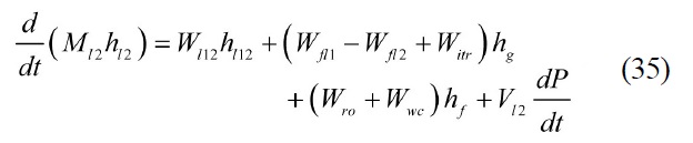
Note that, contrary to conventional pressurizer models, terms for the heater or spray do not appear in the conservation equations. The relationship for mass flow rate between liquid regions is obtained from the requirement that the lower liquid volume is fixed as follows:
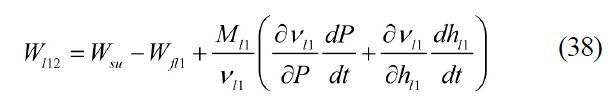
TAPINS employs physical models for local phenomena occurring in the steam-gas pressurizer. The flashing and rainout mass flow rates are calculated by:

where
Dynamic equilibrium, the state in which the condensation rate is equal to the evaporation rate at the interface, is assumed to be at the saturated pressure of the liquid temperature. The coefficient
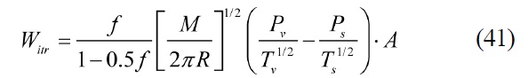
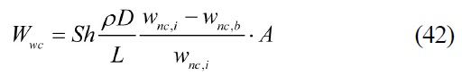
The wall condensate rate in the presence of noncondensable gas is calculated by the analytical model suggested by Kim et al. [33]. In the condensation model, the total heat transfer coefficient is derived from the heat balance at the liquid film interface, and the heat and mass transfer analogy based on mass approach is applied to calculate the condensation heat transfer coefficient in the diffusion layer and the condensate rate. The resultant form for the condensate rate is expressed by:
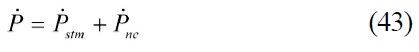
The above conservation equations form a system in which the unknowns outnumber the equations by 11 (4 mass, 4 enthalpy, 3 pressure) to 8. Thus one requires three more constitutive relations for closure. One is the Gibbs- Dalton law for the gas phase, which states that the total pressure exerted by the gaseous mixture is equal to the sum of the partial pressures of steam and nitrogen. With respect to time, this can be expressed as:
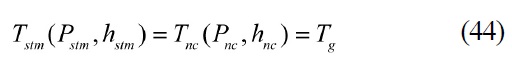
Another constraint is the thermodynamic equilibrium condition in the gas phase. The temperatures of steam and nitrogen, determined by their respective partial pressure and enthalpy, are given by the following:
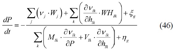
The other relation is the time-dependent pressure equation derived from the constraint on the invariant pressurizer volume with time, which is expressed as:
Note that the
where
See Ref. [10] to check for the detailed expression of
2.4.3 Helical-coil Steam Generator Model
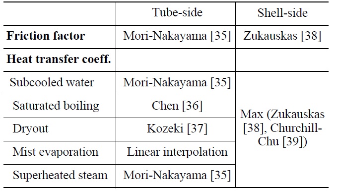
Precise prediction of the heat transport in the helicalcoil S/G is of great importance, especially for free convection flow in an integral system such as REX-10, since the cooling capability of the S/G predominantly affects the stabilized temperature of the primary coolant as well as the transient behavior of the RCS. The steam generator model in TAPINS calculates the shell-side and the tubeside heat transfer coefficients for helically-wound tubes. The heat transfer on the tube-side is estimated using a single helical coil. The heat transfer regions inside the tubes are divided into economizer, evaporator, and superheater sections. Heat transfer and friction factor models similar to those used by Yoon et al. [34], which are employed for the thermal-hydraulic design of a once-through steam generator in SMRAT, are incorporated into TAPINS with slight modifications.
The empirical correlations for the helical-coil S/G in TAPINS are summarized in Table 2. Note that the heat transfer coefficient for the shell-side tube bundles is determined as a larger value between the two calculated by Zukauskas correlation associated with the cross flow across banks of tubes [38] and Churchill-Chu correlation for the external natural convection flow on a horizontal cylinder [39]. By employing the tube-side and shell-side heat transfer coefficients needed to implement boundary conditions for convective flows, the heat conduction equation is solved to predict the transient heat transport from the primary to the secondary circuit.
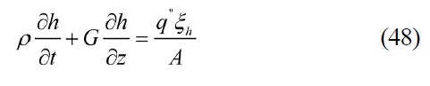
In finding the time-dependent enthalpy-energy distributions along the tube-side of the helical-coil S/G, a simplified approach is applied in TAPINS. The flow rate of the secondary coolant is assumed to be constant, and the following equation is solved for the energy balance:
[Table 2.] Empirical Correlations for Helical-coil S/G in TAPINS

Empirical Correlations for Helical-coil S/G in TAPINS
Eq. (48) is the simplified form of the energy conservation equation. Instead of solving the PDEs for momentum conservation, the three components due to acceleration, friction loss, and gravity are summed to give the total pressure drop along the helical coil. This approach fairly reduces the computational resources with little loss of accuracy in predicting the transient heat transport to the secondary system [10]. In conjunction with the above heat transfer models, the time-dependent heat conduction solutions are advanced across the tubes, which are divided into several intervals.
In TAPINS, the hydrodynamic model is numerically solved using a semi-implicit finite difference scheme on the staggered grid meshes [40]. It has been proved that the semi-implicit scheme is numerically stable and capable of providing an accurate prediction for most applications. In the scheme, the terms associated with the sonic wave propagation are evaluated implicitly. All other terms, including the convection term in the momentum conservation equation, are evaluated at the old time level.
Due to the existence of large momentum sources and sinks in a nuclear reactor, the momentum equation doesn’t have to be necessarily treated in the conservative form. Errors generated by using the non-conservative form are considered to be small and, what is more, the form is more convenient in numerical applications. Thus, the unsteady term and the convection term of the momentum conservation equation can be converted into the non-conservative form by using the continuity equation:
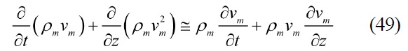
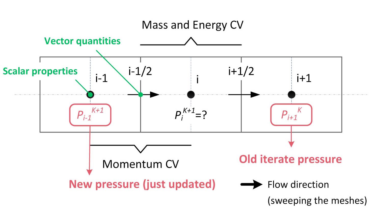
The mesh cell configuration and the labeling convention for cell centers and edges are illustrated in Fig. 5. On the staggered spatial meshes, the scalar properties (pressure, enthalpy, and void fraction) of the flow are defined at cell centers, and the vector quantities (velocity) are defined on the cell boundaries. Thus, the difference equations for
each cell are obtained by integrating the mass and energy equations over the mesh cells from inlet junction to outlet junction. The momentum equation is differenced at the cell edges.
For example, when the mass equation is integrated in a cell, the resultant difference equation expressed in terms of cell-averaged properties and cell boundary fluxes is obtained as follows:
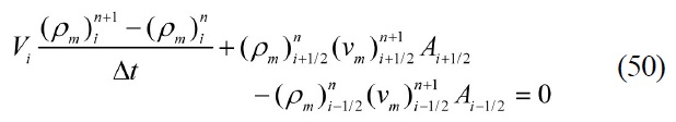
The same procedure is applied to other balance equations, but not presented here. In this scheme, the convective terms in the mass and energy equations, the pressure gradient term in the momentum equation, and the compressible work term in the energy equation all contain terms evaluated at the new time level. All other terms, including the wall friction term and the wall heat source term, are evaluated at the old time level. Because the phase change term Γ
The difference equations of the hydrodynamic model in conjunction with constitutive relations of Section 2.3 represent a nonlinear algebraic system of equations for all mesh variables at the new time level. In TAPINS, void fraction (
In the NBGS technique, all unknowns appearing in the difference equations, except four primitive variables, are eliminated by linearization in terms of the latest iterate values and the four fundamental unknowns. For the mixture mass conservation equation, the mixture density

has to be linearized. From the definition given by Eq. (1), it is linearized as:
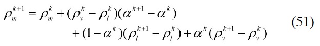
Here, the superscripts are introduced to indicate successive iterative approximations of variables at the new time level. That is,
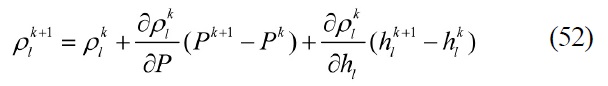
Substituting Eqs. (52) and (53) into Eq. (51) and inserting it into (50) yields the final linear equation for the mass conservation. The above procedure is repeated for the remaining difference equations on the vapor mass conservation and the mixture energy equation. Note that the liquid temperature appearing in Eq. (16) is also linearized in terms of the pressure and the liquid enthalpy for implicit evaluation of the interphase heat and mass transfer in the bulk. Detailed procedures to derive the linear algebraic equations for the four primitive variables are presented in Ref. [10].
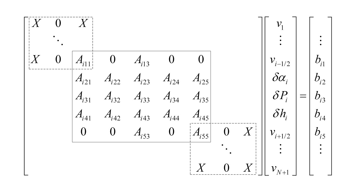
When a linear system based on the above formulations is set up for all the meshes in the loop, the entries of the matrix are arranged in a regular pattern as shown in Fig. 6. The nonzero entries are grouped into a pattern of 5×5 blocks in the linear system. Each of these blocks represents the coefficients of primitive variables for a single mesh cell. The first and fifth rows of the block identify the momentum equations for the inlet and outlet junctions of a cell; the remaining rows are set up from the mixture mass, vapor mass, and mixture energy equations. Note that five variables, including two mixture velocities at inlet and outlet boundaries, for a given cell are coupled only to the pressures in adjoining cells. Thus, if the pressures in the left (upstream) cell and the right (downstream) cell are held fixed, one can solve the 5×5 linear system to obtain the updated primitive variables.
The NBGS method is performed initially by choosing a direction of sweeping the mesh. The unknowns of a given cell are obtained using the new pressure in the left cell but an old iterate pressure in the right cell as depicted in Fig. 5. One can achieve a fast convergence by using the advanced information as soon as it is known in this way. It is noted that the velocity on the boundary between cells is updated twice in this method. This process is continued until the primitive variables in all the cells are updated. The iteration is terminated when the relative pseudo error of pressure is less than a specified value in all meshes. The convergence criterion to be satisfied in TAPINS is expressed as:
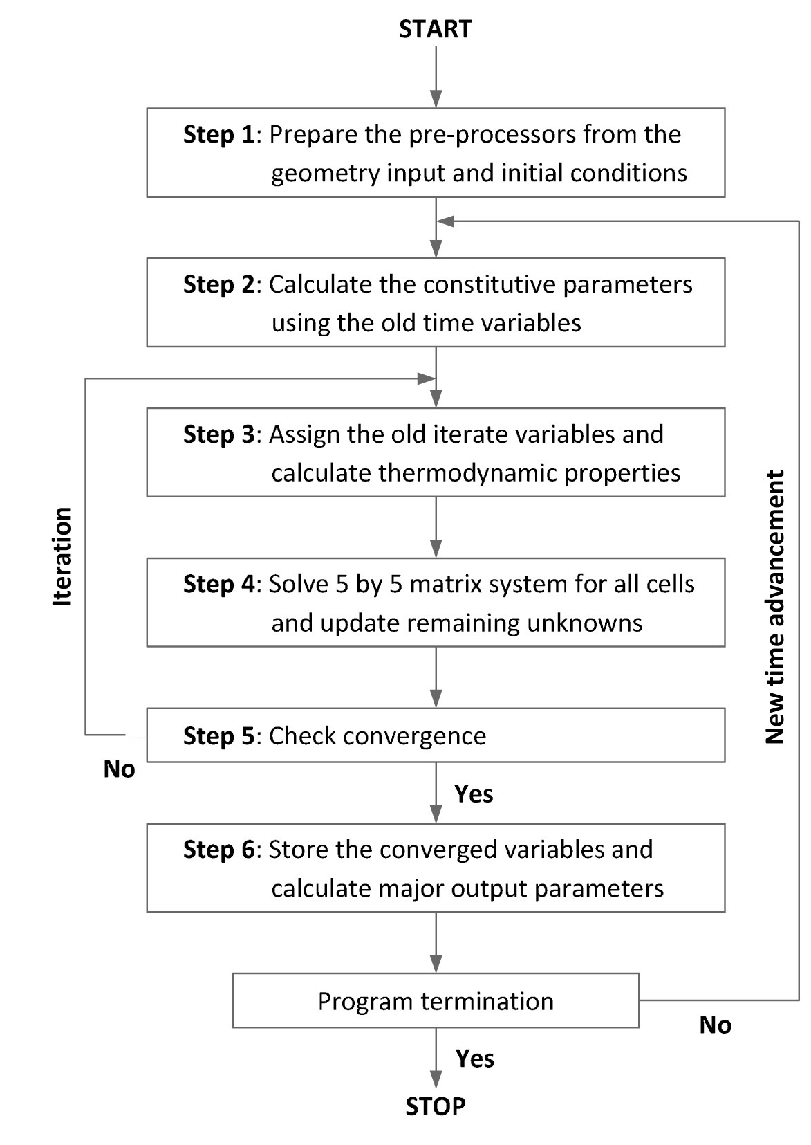
The calculation procedure of TAPINS follows six major steps, as shown in Fig. 7.
Step 1: From the geometry input and the initial conditions supplied by a user, the pre-processors required for the computation are prepared. The fundamental variables are defined and the fluid conditions and properties are initialized.
Step 2: Before getting into the iteration loop, the constitutive parameters for wall-to-fluid heat transfer, wall friction, vapor generation, drift velocity, etc. are explicitly calculated using the old time variables.
Step 3: The iteration loop starts here. The old iterate fundamental variables are assigned to solve governing equations for a mesh cell. Thermodynamic properties are called and the partial derivatives of properties are computed.
Step 4: The 5×5 linear system is solved by Gauss elimination. From the new values for the primitive variables, other remaining unknowns are updated. Steps 3 and 4 are performed for all mesh cells.
Step 5: The convergence test is performed. If the convergence does not succeed, Steps 3 and 4 are repeated unless the iteration number exceeds a specified maximum value.
Step 6: The converged variables are stored and several major output parameters are calculated. Advance to the next time step.
The core and the helical-coil S/G models explicitly evaluate the wall heat sources appearing in the energy conservation equation, and the steam-gas pressurizer model provides the pressure boundary for the field equation solver.
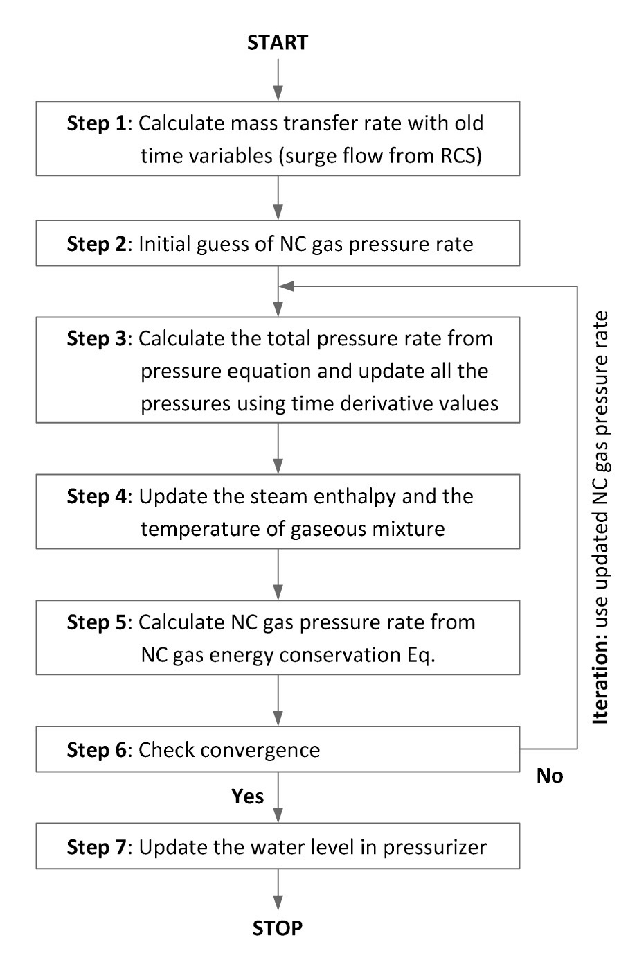
A numerical solution method to facilitate solutions for the steam-gas pressurizer model is also suggested in this study. Since the thermal constraint of Eq. (44) is not a formulated explicit function, but a relation achievable from the steam table, a linear matrix system cannot be established; therefore, the iteration method is employed in obtaining the solutions. Figure 8 shows the flow chart to calculate the transient variation in the total pressure of
[Table 3.] Assessment Matrix of TAPINS based on four-equation DFM [10]
Assessment Matrix of TAPINS based on four-equation DFM [10]
the steam-gas pressurizer. To make a long story short, the guessed pressure rates of each gaseous component, i.e. steam and non-condensable gas, are calculated by using the pressure equation, Eq. (46), and the Gibbs-Dalton law, Eq. (43), and then the convergence is checked by updating these estimations from the energy equations.
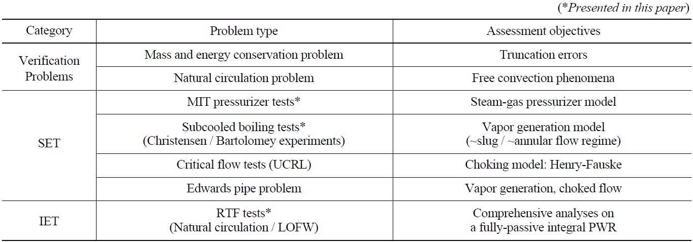
To assess the applicability of TAPINS to thermalhydraulic simulations of integral PWRs, a wide variety of flow situations have been run with TAPINS. The problems for developmental assessment of TAPINS are categorized into three types: verification problems, separate effects experiments, and integral effects experiments. Two simple verification problems are used to demonstrate that the physical equations have been correctly translated into TAPINS [10]. For code validation, a total of 5 calculation sets have been simulated, ranging from steady-state boiling experiments to IET performed in a scaled model of REX-10, RTF.
The verification and validation (V&V) matrix for TAPINS is presented in Table 3 with a brief description on the assessment objectives of each problem. The qualitative and quantitative accuracy of TAPINS is evaluated for problems consistent with the intended application. That is, this assessment matrix is set to validate the mathematical models for thermal-hydraulic phenomena encountered in DBAs of a fully-passive integral PWR such as REX-10. Among the V&V results prepared by Lee [10], aspects of simulations which exhibit the distinguishing features of TAPINS are introduced in this section: analyses on the subcooled boiling test, the pressurizer insurge test in the presence of non-condensable gas, and the change in core power test as well as the LOFW test in the RTF.
The V&V of TAPINS is still ongoing. So far, the assessment of TAPINS has focused on validation works associated with natural circulation and vapor generation. To prove the code correctness, further verification is to be performed with several basic numerical problems, such as those to estimate the pressure drop and the quality, and phenomenological problems. The validation problem of TAPINS will also include the SETs related to the prediction of boiling heat transfer and critical heat flux. For further validation, the SBLOCA test data in the RTF [11] can be utilized to assess the TAPINS capability for two-phase flow processes in an IET facility.
Subcooled boiling is a representative phenomenon associated with the non-equilibrium effect of two-phase flow. Where there is local boiling from the heated surface, vapor bubbles may nucleate at the wall even though the mean enthalpy of the liquid phase is less than the saturated liquid enthalpy. In this phenomenon, the liquid is still subcooled whereas the vapor bubbles are generated regularly at the wall surface and condensed as they slowly move through the fluid. That is, subcooled boiling is characterized by the fact that thermodynamic equilibrium does not exist [41].
The interphase mass transfer and the wall heat flux partitioning model of TAPINS are assessed using the data from subcooled boiling tests conducted by Christensen [42] and Bartolomey [43]. The test section of the Christensen experiment consists of a 127 cm long stainless steel tube with a rectangular cross-section (dimensions 1.11 cm × 4.44 cm). The tube is heated by passing an AC current through the tube walls, and the void fraction along the test tube is measured by a gamma densitometer. In particular, the run No. 15 test is a widely known SET problem used to validate the RELAP5 code [44].
The Bartolomey experiment was performed in a uniformly heated vertical tube of 12 mm in inlet diameter and 1 m in height. Experimental data were obtained at pressures ranging from 3.0 to 14.7 MPa with various heat fluxes, mass fluxes, and inlet liquid temperatures. Regarding these two subcooled boiling tests, a total of four different runs (two from each experiment) are simulated with TAPINS to validate the vapor generation model in the code. The test conditions for the selected sets are summarized in Table 4. For both experiments, TAPINS models the test sections with 20 vertically oriented nodes.
[Table 4.] Test Conditions of Subcooled Boiling Tests Selected for Analysis
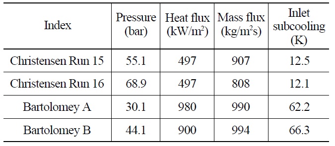
Test Conditions of Subcooled Boiling Tests Selected for Analysis
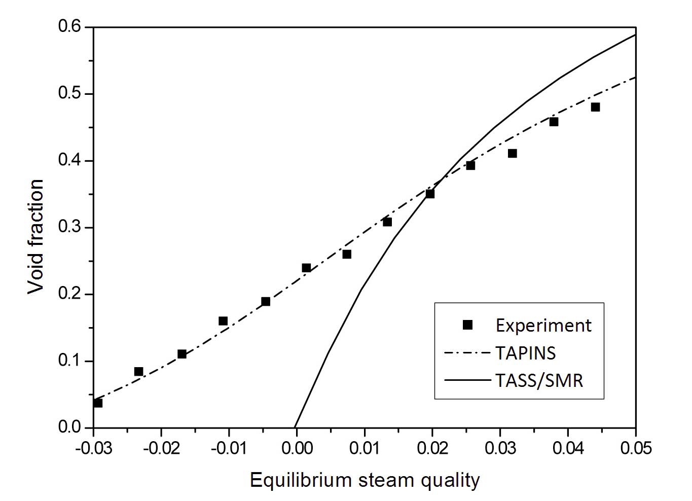
Figures 9 and 10 show the calculation results of TAPINS for the Christensen experiment. In TAPINS, the mass transfer rate per unit volume near a wall is calculated by the Lahey method [18], and the void departure point is predicted by the correlation proposed by Saha and Zuber [19] as stated in Section 2.3.2. Note that the steam equilibrium quality is based on the mixture enthalpy calculated by using the flow quality, not on the mixing cup. The calculated void profiles along the channel agree well with the measured data of Christensen as shown in Figs. 9 and 10. It indicates that the physical model of the interphase mass transfer in TAPINS succeeds in predicting the subcooled boiling phenomena.
The calculation result of the TASS/SMR code for Christensen test 15 is also plotted in Fig. 9 for comparison. As TASS/SMR adopts the homogeneous equilibrium model as governing equations, it cannot predict the vapor generation before the onset of bulk boiling even though there already are significant subcooled voids. In addition, even after the bulk enthalpy is saturated, the prediction of TASS/SMR exhibits some deviation from data. This is because the HEM does not take into account the relative
motion between the phases. Then the predicted void fraction versus the flow quality shows a slight discrepancy with the data even when the mixing cup is the same. It implies that TAPINS may provide more realistic prediction than TASS/SMR on the transients in which non-equilibrium effects are dominant.
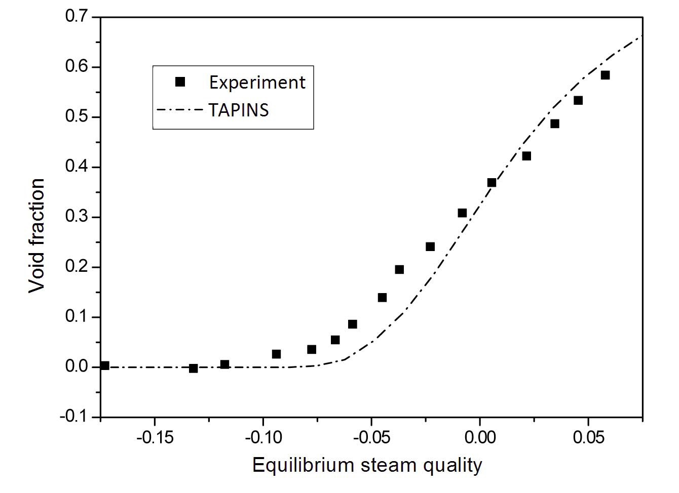
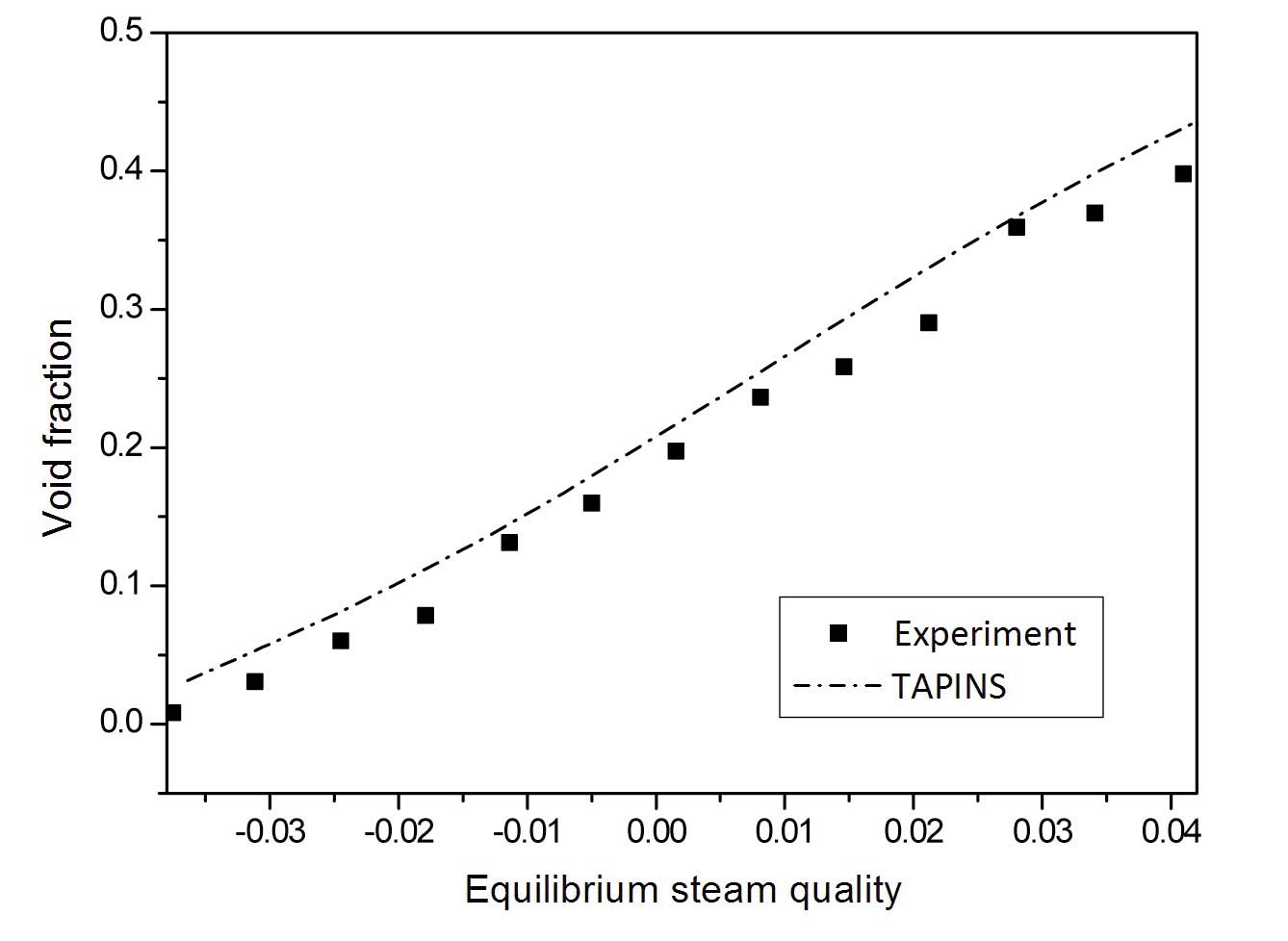
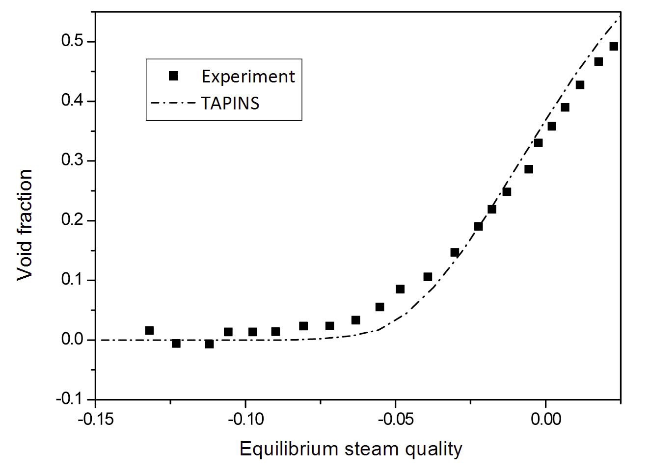
The predicted void fraction profiles of the Bartolomey experiment are plotted in Figs. 11 and 12. While the slug flow regime appears at the exit in the Christensen experiment, the transition to annular-mist flow is encountered in the Bartolomey experiment. The calculation results of TAPINS shows general agreement with the test data of Bartolomey. No sharp break of the profile curve caused by the transition of flow regimes is observed in the calculation results. Moreover, the TAPINS prediction of the void departure point at which the voids begin to be ejected into the subcooled core is almost consistent with the test data of Bartolomey. From the above results, it is revealed that the vapor generation model of TAPINS gives reasonable results for the subcooled boiling phenomena, with an estimated error limit of 0.09 for void fractions in the tests investigated.
4.2 MIT Pressurizer Insurge Tests
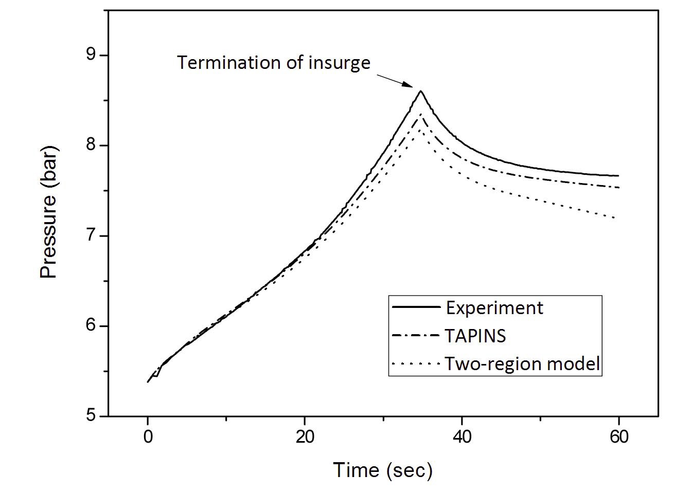
This assessment problem intends to validate the steamgas pressurizer model of TAPINS. Leonard [45] conducted a series of SETs to investigate the response of a smallscale pressurized vessel to insurge transients in the presence of a non-condensable gas. The pressure histories caused by the rapid insurge flow were observed with different types and concentrations of non-condensable gas. The transient is initiated by injecting subcooled water into a primary tank of 0.203 m in inner diameter and 1.143 m in height. The insurge is maintained for approximately 35 s.
Suitability of this SET as a benchmark problem can be explained by the fact that prediction of the pressure response is highly sensitive to local mass transfers inside the pressurizer. Since the volume of the pressurizer vessel is not large (about 0.037 m3) in the test, the amount of vapor filling the test section is correspondingly small. Therefore, the calculation result on the total pressure variation is significantly influenced by the modeling precision of local phenomena. By employing the tests of Leonard as an assessment problem, one can effectively evaluate the accuracies of the proposed governing equations and constitutive relations incorporated in TAPINS. Among the various test cases, two cases of the insurge transient in the presence of nitrogen are simulated with TAPINS, since nitrogen would constitute the gaseous mixture in the steam-gas pressurizer of REX-10.
Figure 13 displays the transient calculation result when the initial mass fraction of nitrogen is 9.7 %. During the insurge, the vessel pressure continuously rises by virtue of the reduction in the gas volume. After termination of the insurge, however, the wall heat transfer from the gaseous mixture results in a moderate decrease in the pressure. The rate of decline slowly decreases as the naturally convective gaseous mixture becomes stagnant after the rise in the water level ceases. Figure 13 reveals that the steam-gas pressurizer model of TAPINS successfully predicts the pressure histories arising from these mechanisms. The deviation of the
calculated final water level from the measured one is at most 1.5 mm.
The accuracy of the three-region model over the tworegion model is also confirmed in Fig. 13. In the simulation of the two-region model, the insurge of subcooled water immediately leads to a decrease in the temperature of an entire liquid region. In actual condition, however, the hot liquid layer, keeping the temperature nearly constant, floats to the top of the liquid region due to thermal stratification. The net effect is that the interfacial mass transfer at the interface into the liquid is over-predicted in the two-region model, causing slight deviation of the prediction results. The three-region model provides a more accurate prediction by reflecting the effect of thermal stratification.
The simulation result when the mass fraction of nitrogen goes up to 20.1 % is plotted in Fig. 14. Compared to Fig. 13, the pressure transient exhibits a steeper slope during the insurge and a higher peak value. It is widely reported that the accumulated non-condensable gas along the wall provides resistance against heat transfer to the wall by condensation. Therefore, the rate of wall condensation is degraded as the concentration of non-condensable gas increases. The TAPINS model predicts the effect of non-condensable gas with reasonable accuracy.
4.3.1 Description of RTF
As mentioned before, one of the distinguishing features
of TAPINS is that it has been assessed by the experimental data from the autonomous IET in the RTF, a scaled-down facility of the prototypical REX-10. The RTF is built to evaluate the characteristics of natural circulation under steady-state and transient conditions and simulate the thermal-hydraulic system behavior during hypothetical accidents [11]. Figure 15 shows the system configuration of the RTF apparatus. Constructed at SNU, the RTF has been designed on the basis of the scaling method proposed by Kocamustafaogullari and Ishii [46]. To provide an identical
hydrostatic head to that of REX-10 for natural circulation, the height ratio is preserved. The volume and power are scaled down by 1/50. In short, the RTF is a full-height full-pressure facility with reduced power.
The primary circuit of the RTF consists of electrical heaters, a riser, four hot legs, a helical-coil heat exchanger, and a pressurizer vessel as shown in Fig. 15. It is designed to operate at full pressure (2.0 MPa) and temperature (200 ℃) with a maximum heater power of 200 kW. The height of the RPV is 5.71 m including the steam-gas pressurizer vessel.
The core region consists of 60 electrical heaters of 1.0 m in the effective heated length. The primary coolant heated in the core passes the long riser and flows into the annular space through the four hot legs. Not appearing in the prototypical REX-10, these elbow-shaped hot legs are set up to install the flowmeters to measure the natural circulation flow rate. The once-through heat exchanger, whose active length is 1.205 m, comprises twelve helical tubes arranged into 3 columns. The innermost, intermediate, and outermost columns are composed of 3, 4, and 5 helical tubes, respectively. The helical coils wrap around the entire annulus between the core barrel and the RPV wall. The primary coolant flows downward across the tube bundles and transfers heat to the secondary coolant flowing inside the tubes.
Located at the lowest region of the RTF is the lower plenum through which most instrumentation around the core is inserted. The pressurizer vessel of 0.381 m in diameter and 0.873 m in height is located on the top of the RTF. In this apparatus, the performance of the steam-gas pressurizer can be simulated by inserting nitrogen into the upper region above the coolant level. See Ref. [10] for more details on the system description, the instrumentation, and the experimental procedure.
4.3.2 Reduction in Core Power Transient
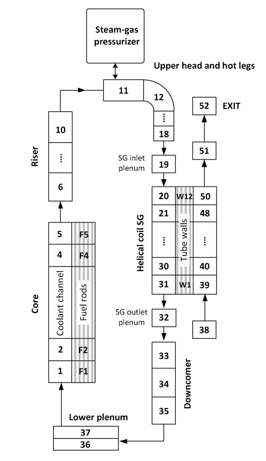
In the TAPINS model of the RTF, a total of 37 nodes constitute the primary circuit; nodes for the core (5), riser (5), upper head including hot legs (8), S/G (14), downcomer (3), and lower plenum (2) establish the RCS of the RTF as illustrated in Fig. 16. The steady-state analysis has revealed that the predictions of TAPINS for the stabilized natural circulation flow rates and the coolant temperatures agree well with the experimental data measured at six different core powers [10]. It indicates that the incorporated S/G model works very well in predicting the shell-side and tube-side heat transfers across the helical tubes.
In this section, the predictive capability of TAPINS is assessed through a comparison with the transient data obtained from the reduction in core power test. One has to remember that the heat transport between the fluid and the internal structures is not trivial in this kind of scaleddown test rig, especially when a dramatic temperature change occurs in the fluid. The stored energy in the structural wall may serve as a heat source during transients, or the
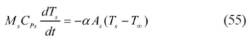
relatively cooler internals may absorb a lot of heat from the fluid. For transient simulations of TAPINS, the heat exchange with the reactor internals is modeled using a lumped approach as follows:
The outer surfaces of the walls are assumed to be adiabatic, and the same heat transfer correlations are used as in the core heat transfer models. The sensitivity study revealed that the modeled coolant flow underwent premature changes in flow rate and temperatures unless the effect of the structural wall was taken into account.
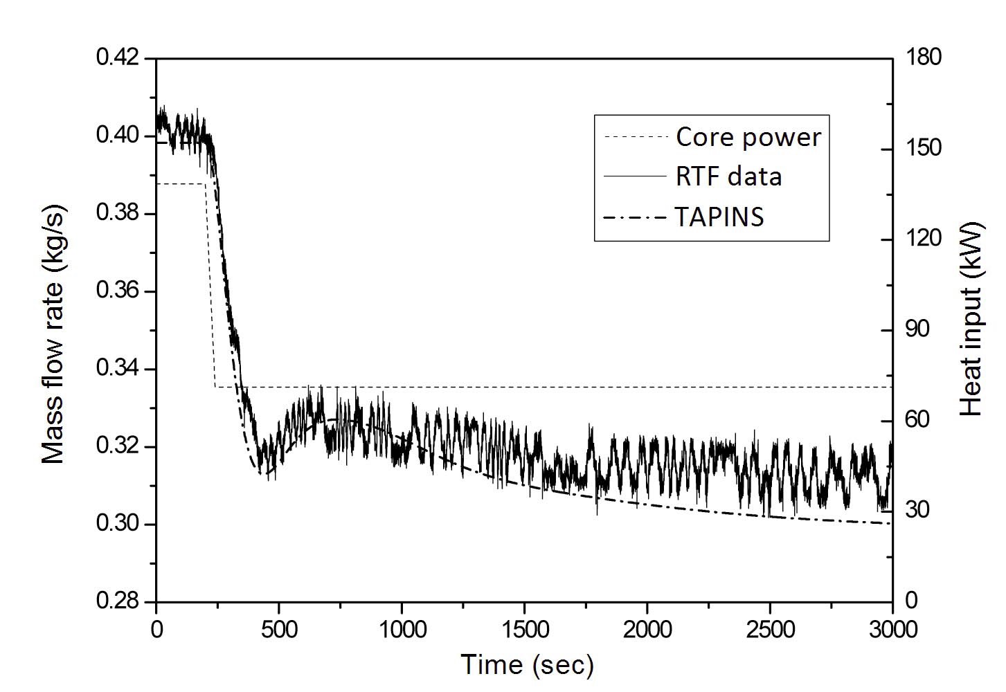
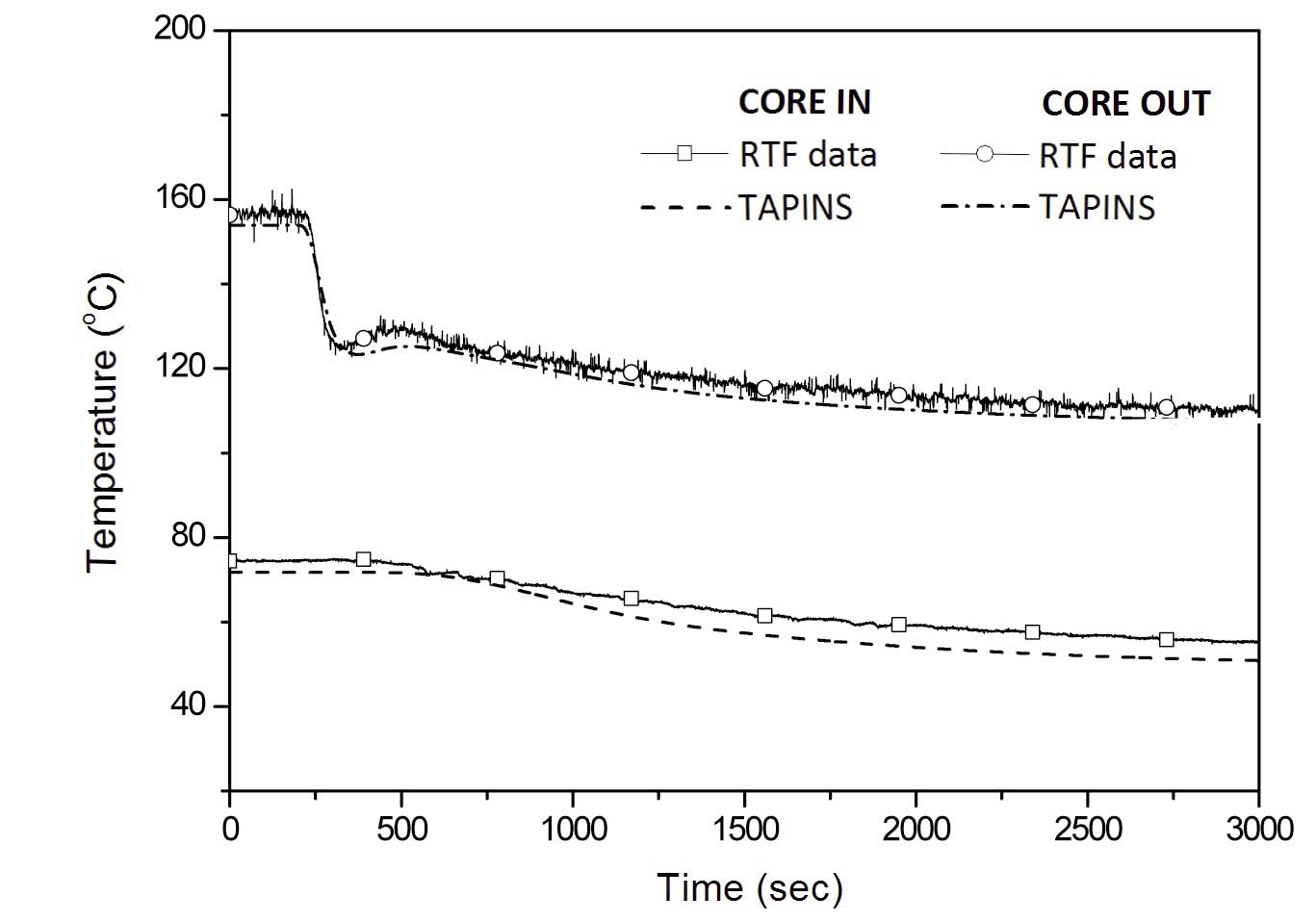
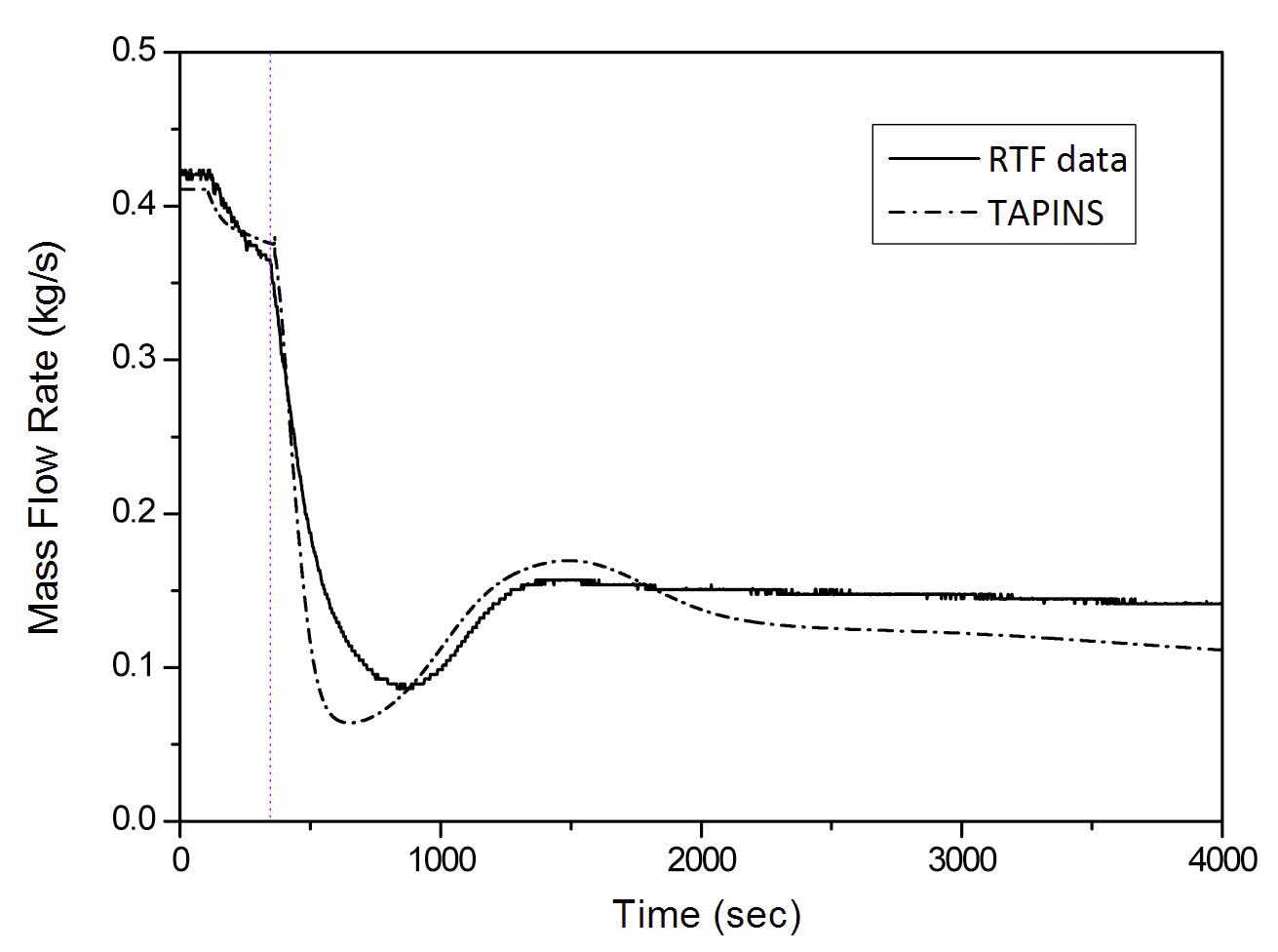
Figures 17 and 18 show the variation of the coolant flow rate and temperatures when the core power drops to nearly half from a stabilized state. At 200 s, the core power is reduced from 138.6 kW to 71.2 kW in a ramp type drop for 40 seconds. In this transient, the reduction in core power is followed by a rapid drop of the natural circulation flow. As the flow velocity is lowered, the temperature rise across the core is somewhat increased, causing a slight overshoot in the coolant flow rate due to the temporary enhancement in the driving force of the free convection. Then the flow rate and the temperatures slowly decrease until a new stabilized state is established. TAPINS succeeds in predicting
the described flow pattern set up by natural circulation and the transient behavior of the coolant temperatures with fine accuracy; deviations of mass flow rate and coolant temperatures are less than 6.4 % and 5.3 K, respectively.
4.3.3 LOFW Accident
The TAPINS application to the LOFW accident of the RTF is presented in this section. This test simulates a hypothetical accident induced by the complete loss of feedwater flow in which the S/G no longer serves as a heat sink until a protective system is actuated. This total loss of feedwater flow can be caused by a mechanical seizure or a power failure of the feedwater pumps, or an inadvertent closure of the feedwater control valves due to malfunction of a feedwater control system [47].
When an actual reactor system is experiences a LOFW accident, the reduced feedwater flow rate immediately triggers the reactor trip. In this test, however, a more conservative scenario is assumed that the low feedwater flow trip is not actuated, but the high pressurizer pressure trip resulting from the coolant heatup leads to reactor shutdown. Once the pressurizer pressure reaches 2.3 MPa, a trip setpoint of REX-10, the heater power is dropped to the decay heat level (about 7%) and the chillers are turned on again to simulate the actuation of the PRHRS. Since the PRHRS is neither established in the RTF system nor designed in detail for REX-10, it is assumed that the natural circulation flow rate of PRHRS is maintained constant at 1/9 of the nominal feedwater flow rate.
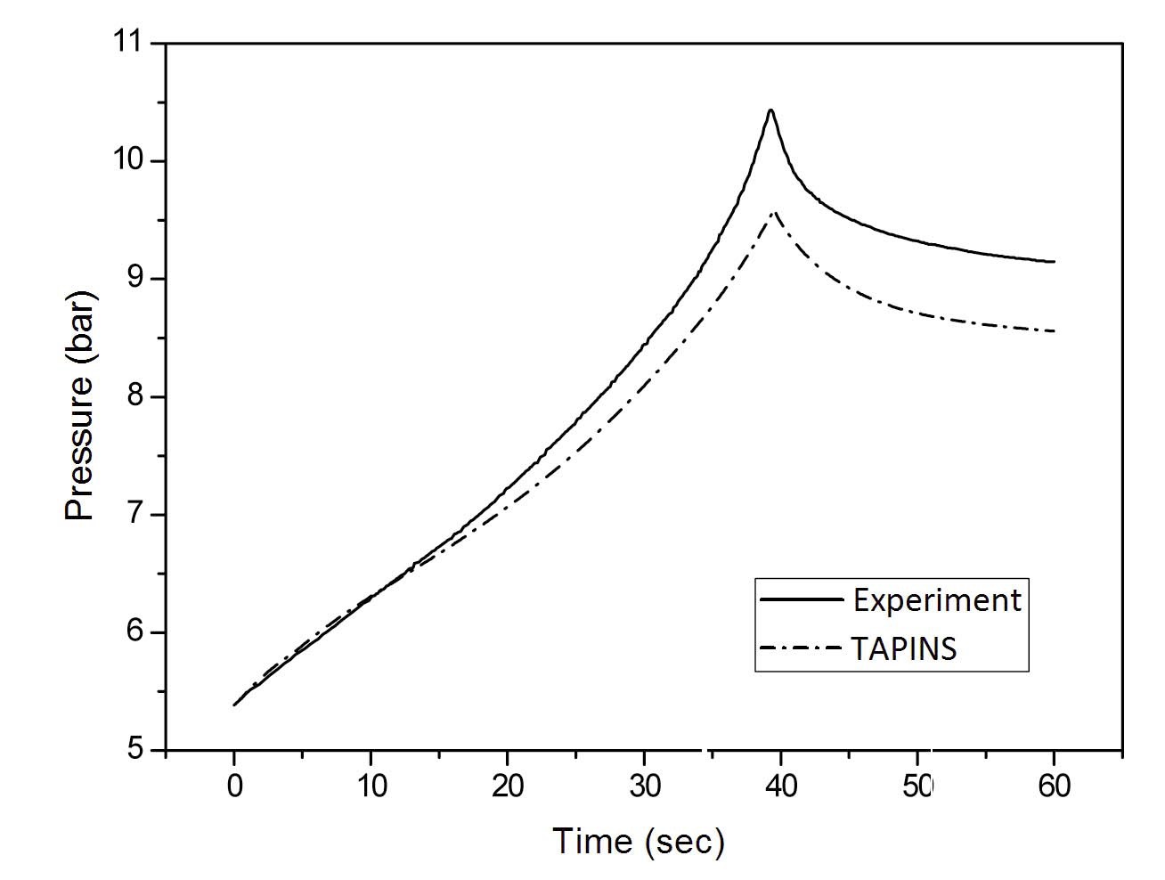
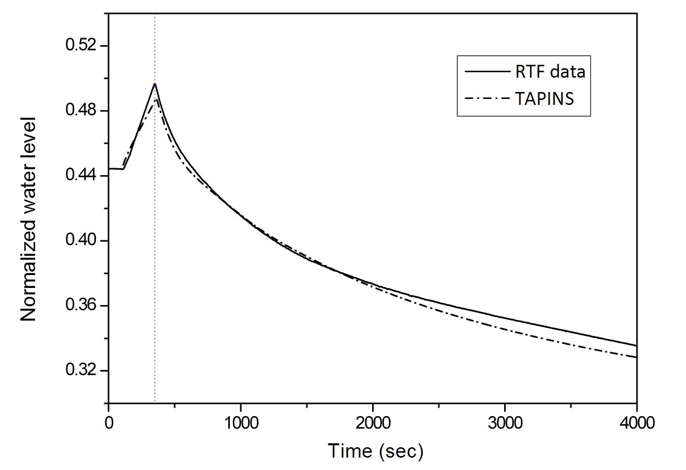
In the analysis of the LOFW accident, the predictive capability on transient response of the steam-gas pressurizer dominantly affects the overall calculation results; if TAPINS fails to predict the accurate moment of the reactor trip under the situation in which the heat removal from the RCS completely vanishes, the calculation results will considerably deviate from the data. The calculation results of TAPINS are shown in Figs. 19 ? 22.
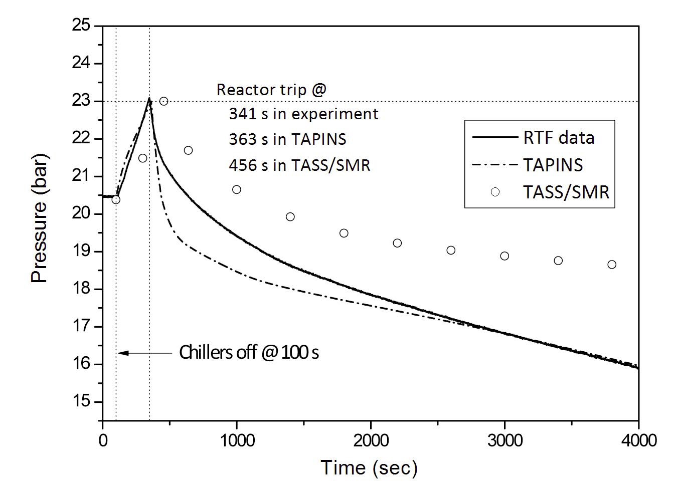
After the chillers are turned off, the coolant is heated up at the rated power as the heat sink vanishes, and the corresponding expansion of RCS coolant and rise in the partial pressure of vapor in the upper gaseous mixture lead to a fast increase in the pressurizer pressure. Due to the absence of a heat sink, the natural circulation flow rate is reduced quite fast as well. The reactor trip occurs 240s after the initiation of transient, and accordingly, the simulated residual decay heat and PRHRS flow is provided. Then the coolant temperatures and the water level in the pressurizer are gradually decreased on account of the continuous cooldown by the PRHRS.
The moment of overpressure trip predicted by TAPINS is about 20 sec later than the experiment. The deviation is not remarkable in view of a long-term transient, which indicates that the steam-gas pressurizer model incorporated into TAPINS provides a reasonable prediction. The calculation result of the pressure transient after the core trip is also consistent with the test data. In addition, the predicted variation in the pressurizer water level is in good agreement with the experiment.
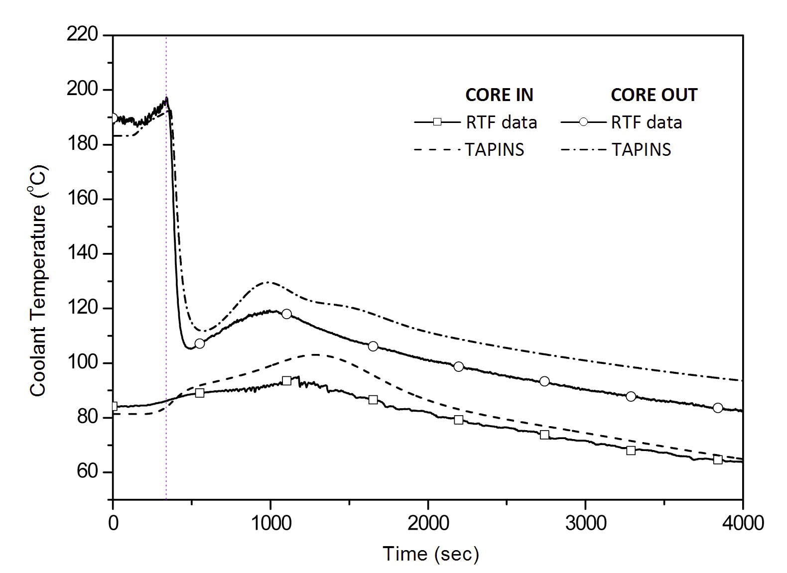
Figures 21 and 22 show the natural circulation flow rate and the change in coolant temperatures in the LOFW accident. The mass flow rate is greatly reduced after the reactor trip, and the RCS coolant is continuously cooled down by the simulated PRHRS function. The results from TAPINS are in general agreement with the data. In a natural circulation regime where the fluid velocity is very low, the calculated flow rate is slightly lower than the measured one. This is attributed to the deviation of the friction factor for low-velocity natural circulation flow, and it also affects the prediction of the coolant temperatures. Since the forced flow correlations are not generally valid in natural circulation flows [48], the friction coefficient models in TAPINS need to be improved to enhance the accuracy.
The calculation results of TASS/SMR on the pressurizer pressure are also plotted in Fig. 19. TASS/SMR predicts that the reactor trip occurs at 356s after the initiation of transient; it is nearly 2 minutes later than measured. Since
the period of the coolant heatup without heat sink is much longer in the calculation of TASS/SMR, it causes significant deviation in overall RCS parameters. From the comparison with IET data of the LOFW accident, it is assessed that TAPINS can provide reasonable prediction on the transient response of the steam-gas pressurizer as well as the RCS behavior of a fully-passive integral PWR.
In order to assess the design decisions and investigate the transient RCS responses of a fully-passive integral PWR such as REX-10, the thermal-hydraulic system analysis code TAPINS has been developed in this study. TAPINS adopts a one-dimensional four-equation drift-flux model for two-phase flow. TAPINS also incorporates mathematical models for the reactor components in an integral PWR. In particular, the new steam-gas pressurizer model based
on the three-region non-equilibrium concept is established and incorporated into TAPINS for better estimation of the pressurizer behavior in the presence of non-condensable gas.
TAPINS is applied to 3 sets of assessment problems to reveal its own distinguishing features. The validation results demonstrate that the calculation results show general agreement with the data, and thus, TAPINS can provide a reasonable prediction of the performances and the transients of an integral PWR operating on natural circulation. Especially, TAPINS can contribute to improved prediction of the transient behaviors of the steam-gas pressurizer.
For practical applications to the SMRs that will be deployed in the near future, TAPINS has to be continuously improved to assure reliable and robust simulations for a wide variety of transients and accidents in a fully-passive integral PWR. In particular, the enhancement of code capability for SBLOCA analysis is essential for TAPINS. Then the improved code capability can be assessed with the SBLOCA experiment in the RTF [11] in the future.
A Cross-sectional area (m2), surface area (m2)
As Heat transfer area of structural wall
Ci Neutron precursor concentration of group i (m-3)
C0 Distribution parameter
Cp Specific heat at constant pressure (J kg-1K-1)
D (hydraulic) Diameter (m), diffusion coefficient (m2s-1)
f Darcy friction factor, condensation coefficient
g Gravitational acceleration (m s-2)
G Mass flux (kg m-2s-1)
h Specific enthalpy (J kg-1)
hcr Critical enthalpy (J kg-1)
hfg Latent heat (J kg-1)
H Volumetric heat transfer coefficient (W m-3K-1)
j Superficial velocity (m s-1)
L Length (m)
M Mass (kg), molecular weight (kg mol-1)
N Neutron density (m-3)
P Pressure (Pa)
? Time derivative of pressure (Pa s-1)
q" Heat flux (W m-2)
R Universal gas constant (J mol-1K-1)
Sh Sherwood number
t Time (s)
T Temperature (℃)

Core-averaged temperature (℃)
u Velocity (m s-1)
ub Bubble terminal velocity (m s-1)
ud Liquid drop velocity (m s-1)
v Velocity (m s-1)
V Volume (m3)

Drift velocity (m s-1)
w Mass fraction
W Mass flow rate (kg s-1)
z Spatial coordinates (m)
Greek Letters
α Void fraction, heat transfer coefficient (W m-2K-1)
αT Reactivity temperature coefficient (K-1),
β Total delayed neutron fraction
βi Delayed neutron fraction of group i
Γ Phase change rate (kg m-3s-1)
Δhgf Enthalpy difference between phases (J kg-1)
Δρ Density difference between phases (kg m-3)
ε Pumping term
Λ Neutron generation time (s)
λi Decay constant of precursor group i (s-1)
ν Specific volume (m3 kg-1)
ρ Density (kg m-3), reactivity

Core-averaged density of coolant (kg m-3)
σ Surface tension (J m-2)
ξh Heated perimeter (m)
Subscripts
b Bulk properties
ext Externally introduced
f Fuel, saturated liquid
g Saturated vapor, gaseous mixture in pressurizer
i Delayed neutron precursor group, interface, noding index
if Bulk interface for liquid
ig Bulk interface for vapor
in Insertion of non-condensable gas into pressurizer
l Liquid phase
l1 Lower liquid region of pressurizer
l2 Upper liquid region of pressurizer
l12 Between lower and upper liquid regions
m Mixture, moderator
nc Non-condensable gas
r Relative difference between phases
rv Relief of gaseous mixture
s Structural wall, saturated state
sgp Steam-gas pressurizer
stm Steam
w Wall
v Vapor phase
0 Initial values
∞ Free stream condition
Superscripts
k Iteration step
n Time level index
s Saturation property


![Assessment Matrix of TAPINS based on four-equation DFM [10]](http://oak.go.kr/repository/journal/12587/OJRHBJ_2013_v45n4_439_t003.jpg)