To communicate with a ground station, a satellite on low-Earth orbit is equipped with an omnidirectional or a directional antenna system. When a satellite is equipped with a directional antenna system, a gimbal system is included in the antenna system, to change the antenna-pointing vector. Korea multi-purpose satellite-3 (KOMSAT-3) is the third satellite developed by the Korea Aerospace Research Institute (KARI) to observe the Earth’s surface. To transmit stored images from the satellite to a ground station, KOMSAT-3 is equipped with a directional antenna system that includes a 2-axis gimbal system [1]. The tracking profile (TP) for the azimuth and elevation angles of the gimbal system is scheduled from the ground station in advance, and the information related to the TP is transmitted to the satellite’s on-board computer. The tracking profile is reconstructed in the flight software, and the antenna-pointing vector is controlled along the tracking profile, to communicate with the ground station.
The tracking profile design is based on the satellite attitude, mission orbit, and position of the ground station. The satellite attitude is scheduled as an attitude profile in a higher operational level. Generally, the attitude profile for an Earth observation mission can be divided into several segments, which can be categorized into two phases. One of the two phases is an imaging phase, for taking images of the Earth’s surface; the other is the maneuver phase, for reorienting the satellite attitude toward the next target point. Depending on the object of the Earth observation mission, the attitude profile is composed of several sequences of imaging phase and maneuver phase. In the imaging phase, to acquire images of better quality, the motion of gimbal angles must be minimized. Therefore, in the process of designing the tracking profile of the gimbal angles, the motion of the gimbal angles in the imaging phase should be taken into account.
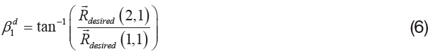
In Refs. [1-2], the desired azimuth and elevation angles were extracted from the desired antenna vectors, which were the directions of the antenna-pointing vectors oriented directly to the ground station. Based on the desired gimbal angles, the tracking profile was designed by the least-square method with polynomials.
In [3], a tracking profile was optimized by a reinforcement learning algorithm. The results of Ref. [3] revealed that because a directional antenna has a specified beam-width, pointing exactly at the ground station was not necessary for the antenna-pointing vector. However, in [3], even though the designed profile satisfied the beam-width constraint, the motions of the gimbal angles were not minimized in the imaging phase.
In [4], a tracking profile for directional antenna was designed using a virtual ground station. Based on the algorithm proposed in Ref. [4], the angular velocity for the gimbal angle was decreased by choosing a fixed position of the virtual ground station in the Earth Centered Earth Fixed frame. However, how to choose the fixed ground station properly was not explained.
This paper considers the tracking profile design problem. In this paper, the virtual ground station is not a fixed point, but a moving point, which is designed automatically through the tracking profile design process. For this goal, the design process is composed of two steps. First, to minimize the motion of the gimbal angles in the imaging phase, each antenna tracking profile corresponding to each imaging phase is generated. After generating tracking profiles in the
imaging phase, the tracking profiles in the maneuver phase are designed. For this goal, two optimization-problems are formulated.
The remainder of the paper is organized as follows. First, the way to calculate the desired antenna vector and the desired gimbal angles is explained, and the previous approaches to generating antenna tracking profiles are reviewed. After these explanations, the proposed algorithm is introduced, and numerical examples are presented.
2.1 Desired antenna-pointing vector/gimbal angles
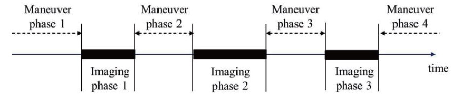
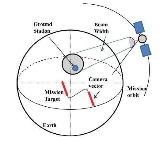
Fig. 1 shows an example of the mission sequence for the Earth observation satellite. The imaging phase is the phase in which images of the Earth’s surface are taken. And the maneuver phase is the phase in which an attitude reorientation maneuver is executed, for orienting the line of sight vector of a payload to the starting point of the next imaging phase. To accomplish these kinds of mission sequences, attitude profiles should be designed in advance, using target positions of the Earth’s surface, and satellite positions on the mission orbit. Even though the ground station is fixed in the Earth-Centered Earth-Fixed (ECEF) frame, because the attitude of the satellite is controlled along with the attitude profile, and the satellite also revolves around the Earth, the position vector of the ground station is a time-varying vector, with respect to the satellite body frame. Therefore, if a directional antenna is equipped on the satellite, a gimbal system is required to communicate with a ground station. In this paper, a 2-axis gimbaled antenna system is assumed to be installed on the satellite.
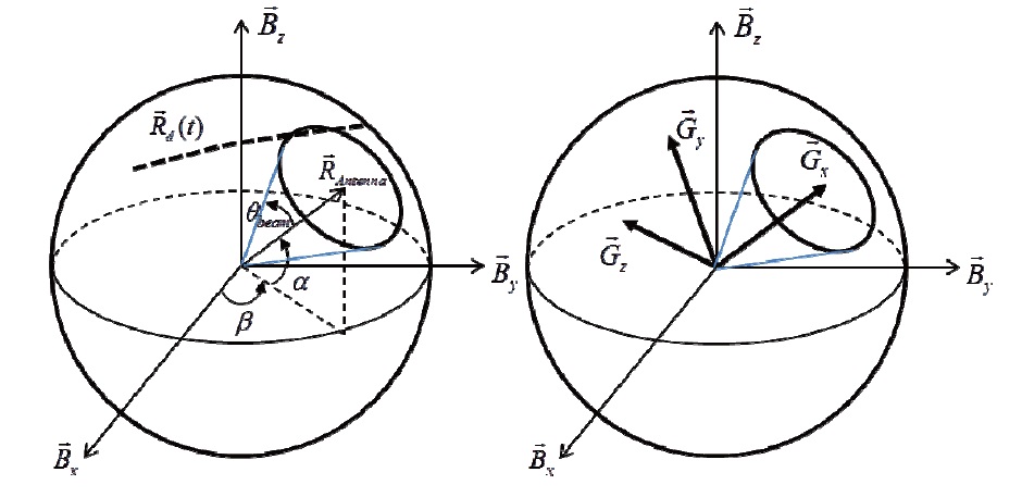
A conceptual diagram of the antenna tracking profile design problem is depicted in Fig. 2. In Fig. 3, the problem is illustrated in the satellite body frame.
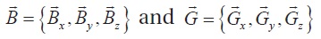
are the body frame and the gimbal frame coordinate, respectively. Initially, the gimbal frame is aligned to the body frame.

and the azimuth angle about the

is not unbounded; whereas the rotation-axis for the elevation angle is aligned to the

and the elevation angle is bounded between a lower bound

denotes the time-varying position vector of the ground station in the body-frame, and

is the pointind vector of the antenna.
can be computed as follows.
denote the position vectors of the satellite and the ground station in the ECEF-frame, respectively. Using
the normalized position vector from the satellite to the ground station is calculated as follows;
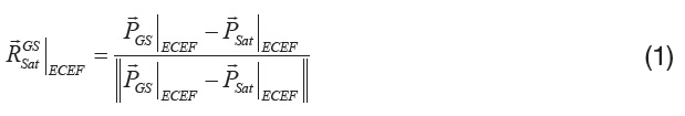
Where,

is the normalized position vector from the satellite to the ground station. The vector defined in the ECEF-frame can be transformed into the vector defined in the satellite body-frame using a direction cosine matrix, which can be calculated by the information of the satellite
attitude and orbit, as follows:

Where,

are the direction cosine matrices, which transform a vector from an Earth Centered Inertial (ECI) frame, respectively. Because the orbit data and the attitude profile are continuous, a continuous vector trace for

can be generated. In this paper, the vector of
is considered as the desired vector of.

If the azimuth and elevation angles are given, the pointing vector from the center of antenna can be calculated as follows.
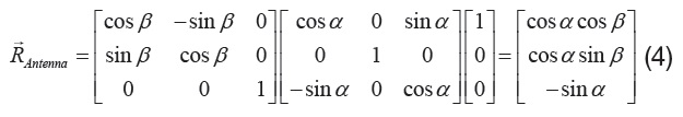
Using Eqs. (2)-(4), the antenna gimbal angles corresponding to the desired vector
can be calculated. The antenna gimbal angles corresponding to the desired vector
are denoted as
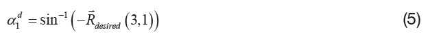
And the second set is denoted as (


In the previous papers [1-4], only the first set of desired angles in Eqs. (5)-(6) was considered in the tracking profile design process. Designing the tracking profile using only one set between two sets may increase the angular velocity of the gimbal angles, if some vectors near the vector of [0 0 1]T are included in the desired gimbal vectors. If two sets are considered in the process of tracking the profile design, the angular velocity of the gimbal angles can be efficiently decreased, which will be shown in the numerical example section.
2.2 Previous approaches to design of the antenna tracking profile
In the previous section, the ways to calculate the desired vectors and gimbal angles were explained. The desired gimbal angles can be calculated at user defined sampling points. However, uploading all the desired gimbal angles is not appropriate, because the amount of data is too large. Therefore, the desired gimbal angles are approximated with polynomials, and the coefficients of the polynomials are uploaded from the ground station. The antenna tracking profile is reconstructed in the onboard flight software using the uploaded coefficients. In Refs. [1-2], each gimbal angle was approximated by


Where,
are the coefficients of the polynomials. Let
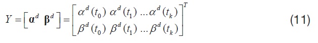
The approximated gimbal angles at the sampling points can be organized in a matrix form, as follows.
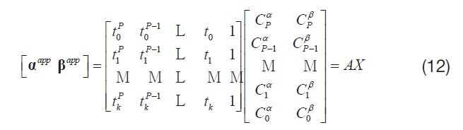
In the previous approaches [1-2], the least-square method was used to determine the coefficients of
where,

Using the virtual ground station instead of the true ground station, an alternative approach is suggested in Ref. [4]. In this approach, the least-square to determine the polynomial coefficients was also applied. The above approaches are simple and can be easily implemented. However, the approaches could not handle the mechanical or operational constraints, such as gimbal angle, angular velocity, and constraints related to the beam-width angle. In particular, using these approaches, the magnitude of the angular velocity in the imaging phase could not be minimized.
3.1 Parameter Optimization Problem
In this paper, the antenna tracking profile will be designed with the polynomials and coefficients. The coefficients of the antenna tracking profile will be optimized, by solving parameter optimization problems. Because the main object is to minimize the motion of the gimbal angles at each imaging phase, the antenna tracking profile for each imaging phase will be separately designed. After designing the tracking profile in the imaging phase, the tracking profile in the maneuver phase is sequentially designed. The object for the antenna tracking profiles design problem in the maneuver phases is to make smooth paths between two tracking profiles of the imaging phases. If there are
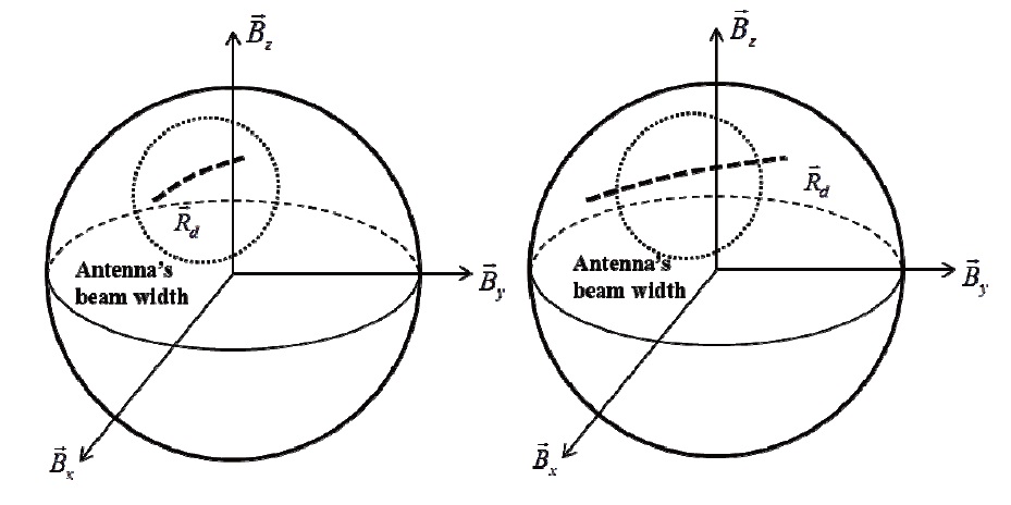
The ideal result for the antenna tracking profile in each image-phase is that azimuth and elevation angles are to remain as constant values, which means that angular velocities and angular accelerations are zeros. At the same time, the desired antenna vector lies within the beamwidth. However, it may not always be possible. Consider two cases, as shown in Fig. 4. Fig. 4 shows two examples of the geometric relations between the desired antenna vectors and the beam-width. The left figure in Fig. 4 shows that the overall desired antenna vectors in the
Approximately, to decide whether the given desired vectors in the
is calculated, as follows.
Where,
are the sampled desired vectors in the
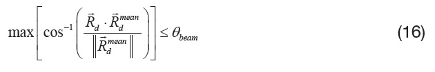
If Eq. (16) is satisfied, the tracking profile in the
gimbal angles using

If Eq. (16) is not satisfied, motions of the gimbal angles are assumed to be necessary. Under this case, the following parameter optimization problem is considered, to design the gimbal angle profiles. The angular velocities of the gimbal angles are assumed to be constant at the

Where,


Where,
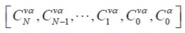
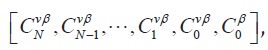
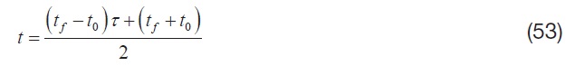
be the times corresponding to the sampled points. Then, the gimbal angles, angular velocities, and angular accelerations at the sampled points can be arranged in a vector form, as follows.


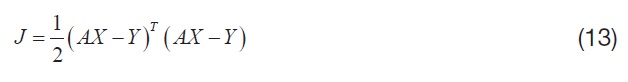
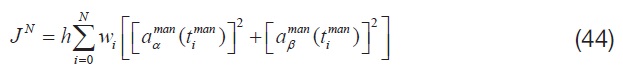
In this paper, the main objective is to minimize the motion of gimbal angles, which may produce mechanical vibration and reaction torque to the satellite at the imaging phases. Because the angular accelerations of the gimbal angles are zero, the reaction torque generated from the gimbal system can be negligible. Therefore, to minimize the motion of the gimbal angle, the following cost function related to the angular velocity of the gimbal angles is considered.

The parameter optimization problem is summarized as follows: finding the constant angular velocities and the initial gimbal angles of [


Eq. (30) is the inequality constraints related to beamwidth constraints. In Eqs. (32)-(33),
are the maximum allowed angular velocities, given as the mechanical constraints at the imaging phase.
To design the antenna tracking profiles at the maneuver phase, the angular velocities of the gimbal angles are organized with P-order polynomials.


Where,
are the polynomial coefficients to be optimized. From Eqs. (34)-(35), the gimbal angles can be calculated as follows.


Let t


As commented in previous subsection 3.2, angular acceleration of the gimbal angles may produce reaction torque to the satellite, according to the principle of the conservation of angular momentum. Even though the reaction torque can be cancelled by the attitude control system, a smaller reaction torque is preferable, from the attitude control accuracy point of view. Because the reaction torque has a close relation to the gimbal acceleration, the following cost function is considered to generate a smooth path in the maneuver phases.
Where,
Where,


Finally, because the antenna-pointing vectors reconstructed from the designed azimuth and elevation angles by utilizing Eq. (4) are required to be within beamwidth, the following inequality constraint is also imposed.

The parameter optimization problem for the maneuver phase is summarized as follows: to find polynomial coefficients of the angular velocity profiles at the maneuver phase and initial gimbal angles
and
[Table 1.] Mechanical/operational constraints for the gimbaled antenna system
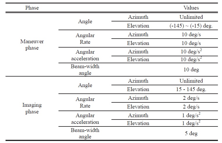
Mechanical/operational constraints for the gimbaled antenna system
to minimize the approximated cost function in Eq. (44), while satisfying Eqs. (45)-(52).
In the paper, the Legendre-Gauss-Lobatto (LGL) points are considered as the sampling points. Let

which is the derivative of the Legendre polynomial
The integral of a function

where,
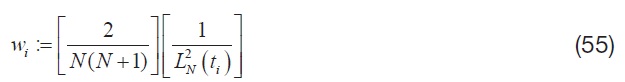
Therefore, the weight
In this section, numerical examples are presented. In this paper, the beam-width angle for the directional antenna system was assumed to be 10 degree. However, a different magnitude of beam-width angle was applied in the problem. In the maneuver phases, 10 degree of beam-width angle was considered; however, in the imaging phase, 5 degree of beam-width angle was considered strategically. The mechanical or operational constraints for the gimbal system considered in this paper are summarized in Table 1.
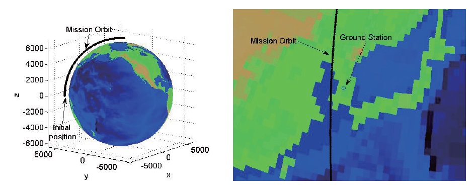
A Sun-synchronous orbit with altitude of 550 km was considered as the mission orbit. The data for the mission orbit were generated by Satellite Tool Kit (STK). Two imaging phases were assumed to be the purpose for the mission. Daejeon in the Republic of Korea was chosen as the position of the ground station (GS). Fig. 5 shows the initial position of the satellite, the mission orbit, and the position of the ground station in the ECEF frame.
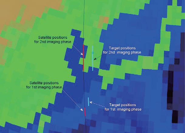
From the initial time corresponding to the initial position, the first and second imaging phases were assumed to be executed at 440 sec and 540 sec with a duration of 19 sec and 59 sec, respectively. In Fig. 6, the satellite positions for the imaging phases, and the target positions to be taken on the Earth surface are marked.
To take images for the target positions, the attitude profile is required to be designed in advance. For the above mission,
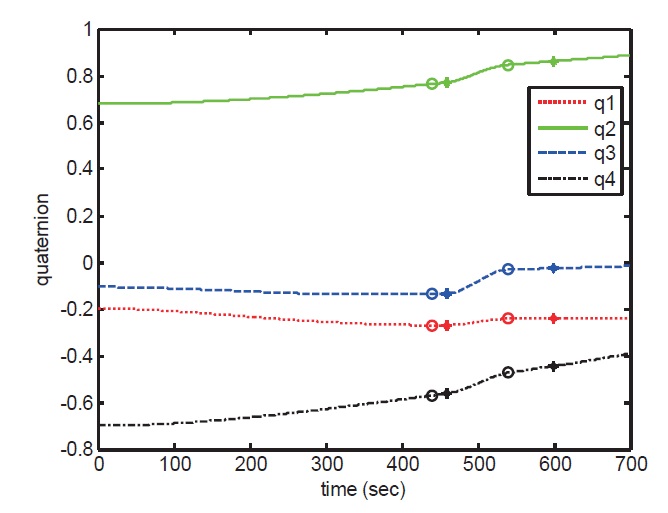
the attitude profile was designed using the algorithm presented in Ref. [7]. The attitude profile corresponding to the above mission is presented in Fig. 7. In Fig. 7, the marks of ‘o’ and ‘*’ depict the start time and the end time of each imaging phase. If the mission orbit, the attitude of the satellite, and the position of the ground station are given, the unit position vectors of the ground station in the body frame can be calculated using Eqs. (1)-(2). As commented in the previous section, the unit position vectors of the ground positions in the body frame are the desired antenna vectors.
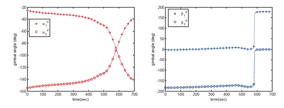
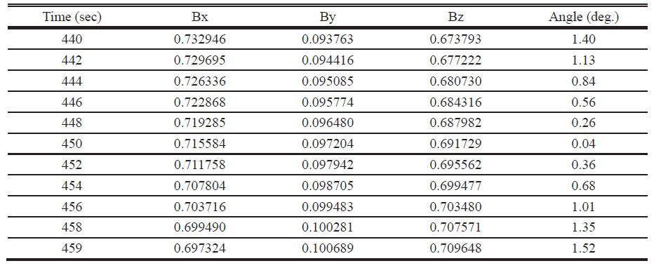
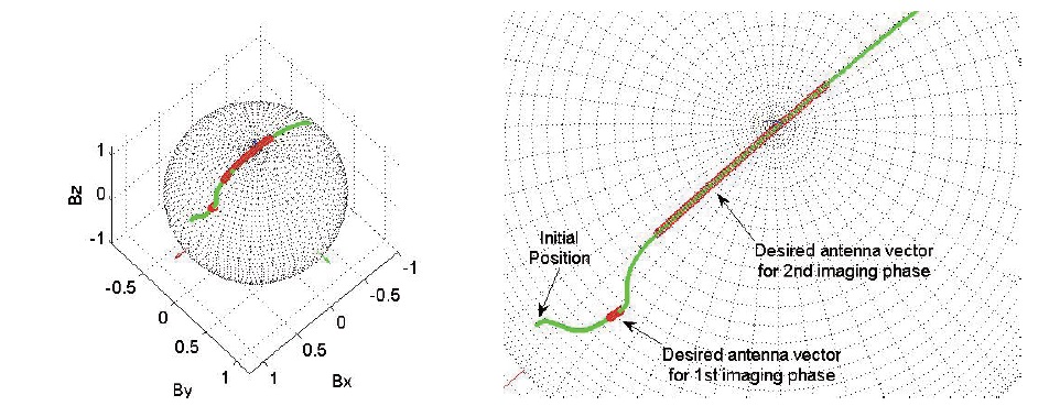
In Fig. 8, the desired antenna vector is presented on the unit sphere in the body frame. The desired antenna vectors at the 1st and 2nd imaging phases are illustrated with a distinguishing line style. The desired antenna vectors were computed at every second, and portions of the desired vector at the imaging phase are presented in Tables 2 and 3. The two-set of desired gimbal angles were calculated by Eqs. (5)-(8), and the desired gimbal angles are presented in Fig. 9. In this example, some vectors close to [ 0 0 1]T were included. Because the vector of [ 0 0 1]T is a singular vector, the azimuth angle corresponding to the vector of [ 0 0 1]T cannot be defined. Therefore, if the vector of [ 0 0 1]T is included in the desired vector, a jump in the desired azimuth angle history happened. If some vectors around the vector of [ 0 0 1]T were included in the desired vector history, a sharp change in the history of desired gimbal angles can be seen in Fig. 9. Therefore, designing a tracking profile using only one desired gimbal angle set between two sets is not appropriate.
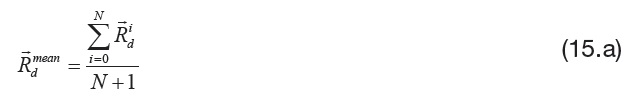
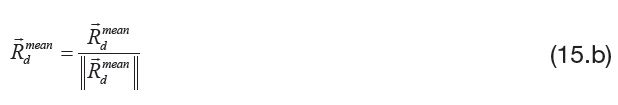
Using the desired vectors as shown in Fig. 8, the unit mean vector was computed by Eq. (15). The unit mean vector was computed as follows:
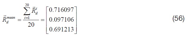
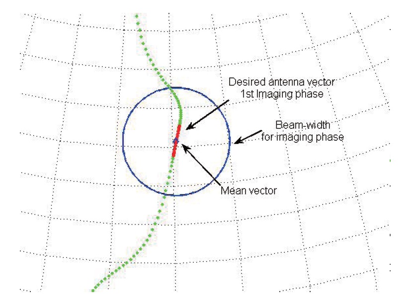
The angles between the unit mean vector and the desired antenna vector are presented in the fifth column of Table 2. The maximum value among the angles is 1.52 degree, which is smaller than the 5 degree of the antenna beam width angle. Therefore, it was concluded that the desired antenna vectors lie within the beam-width. The desired antenna vectors, unit mean vector, and beamwidth are presented in Fig. 10. As shown in Fig. 10, the desired antenna vectors are within the beam-width,
[Table 2.] Desired antenna vectors at the 1st imaging phase

Desired antenna vectors at the 1st imaging phase
whose center is the unit mean vector. The antenna tracking profile in the first imaging phase can be chosen as the stationary vector of [0.716097 0.097106 0.691213]T, which is the same as the unit mean vector. The elevation and azimuth angle corresponding to the stationary vector were computed as -43.7262 degree and 7.7226 degree from Eqs. (5)-(6).
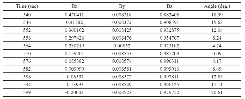
Using the desired antenna vectors in the second imaging phase, the unit mean vector was computed by Eq. (3), as follows:
[Table 3.] Desired antenna vectors at the 2nd imaging phase

Desired antenna vectors at the 2nd imaging phase
[Table 4.] Boundary conditions in the optimization problem for the maneuver phases
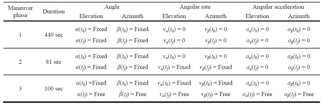
Boundary conditions in the optimization problem for the maneuver phases
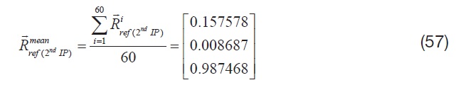
The angles between the unit mean vector and the desired antenna are presented in the fifth column of Table 3.
The maximum value among the angles is 20.61 degree, which is larger than the antenna beam width angle of 5 degree. Fig. 11 shows the relation between the unit mean vector and the desired antenna vectors. Therefore, the antenna tracking profile at the 2nd imaging phase was approximated as a first-order polynomial, as Eqs. (19) and (20). The coefficients of
Therefore, the designed antenna tracking profile for 540≤


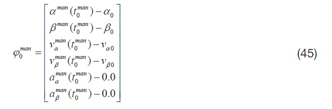
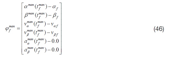
At
as the boundary conditions of the gimbal angles, in the optimization problem of the maneuver phases.
There are three maneuver phases in this example. A 7th-order polynomial was used for each tracking profile in the maneuver phase. In each optimization problem, the boundary conditions were chosen to connect the antenna tracking profiles of the imaging phases, which are listed in Table 4.
For example, in the optimization problem for the second maneuver phase, the boundary conditions for the initial azimuth and elevation angles were chosen as the final gimbal angles of the antenna tracking profile in the first imaging phase. And the boundary conditions for the final azimuth and elevation angles were chosen as the initial angles of the antenna tracking profile in the second imaging phase.
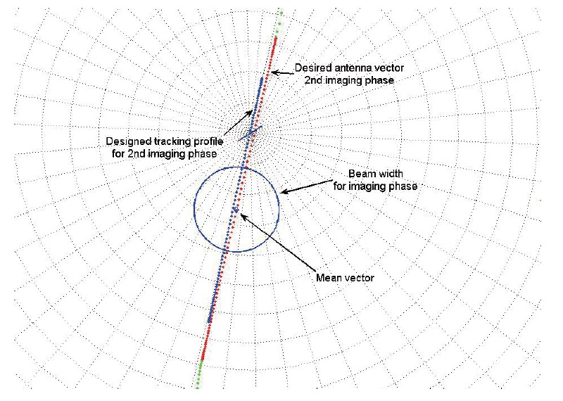
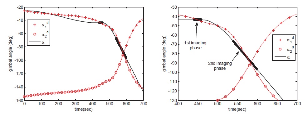
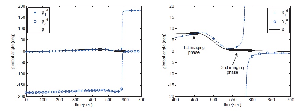
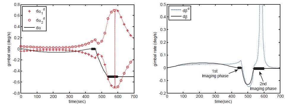
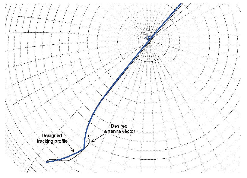
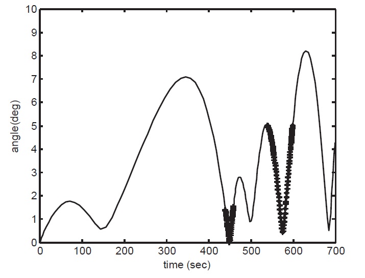
The parameter optimization problems were also solved by the ‘fmincon’ function implemented in @MATLAB. Figs. 12-16 show the optimization results. Figs. 12-13 are the results for the designed gimbal angles with the two-set of desired gimbal angles. Marks ‘+’ and ‘o’ stand for the two sets of desired gimbal angles. As shown in Figs. 12-13, the tracking profile was designed smoothly between the two sets of desired gimbal angles. In this paper, two possible desired gimbal angle sets were not used directly, but the desired vector was used. The approach used in this paper can automatically make a continuous tracking profile between two sets of desired gimbal angles. This result was not found in previous researches. Fig. 14 shows the results for the gimbal angular velocities. Also, the profile of the angular velocity was continuously connected. As shown in Fig. 14, it was confirmed that the angular velocities were zeros for all the first imaging phase. In Fig. 15, the overall desired antenna vectors and designed tracking profile are presented on the unit sphere in the body frame. Furthermore, Fig. 16 shows the result related to the beam-width constraint. The angle differences between the desired antenna vectors and designed antenna vectors were less than 10 degree of beamwidth angle, which means that the beam-width constraints were satisfied.
In this paper, parameter optimization problems were formulated to design antenna tracking profiles. In the optimization problems, mechanical constraints, such as the bounds for gimbal angles, angular rates, and angular accelerations, were taken into account. The main objective was to minimize the motion of the antenna’s gimbal system during the imaging phase. Our study confirmed that if a trace of the desired vector was within the given beam-width angle, the motion of the gimbal angles was not required. If motion of the gimbal angles was required, the profile of the azimuth and elevations angles could be successfully designed with a first-order polynomial. Even though a first-order polynomial was used in this paper for the tracking profile in the imaging phases, high-order polynomials can also be used. To connect the antenna tracking profiles between the imaging phases, another optimization problem under boundary conditions was solved in the maneuver phase. Through numerical examples, it was verified that the overall tracking profile could be continuously designed, and the motions of
the gimbal system in the imaging phase could be drastically minimized.