e Integration of overload error

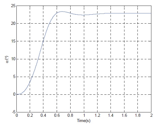
α Angle of attack of interceptor

ωz Pitch angle rate of interceptor

aij Aerodynamic force coefficients and aerodynamic moment coefficients

v Speed of interceptor

g Acceleration of gravity

nzc Command of overload

A State matrix

B Control matrix

x System state vector

u Control input vector

K State feedback controller

Sat(.) Saturation limitation

ρ Saturation value of the Rudder deflection angle or angle rate

P,W,G,H Positive definite matrices

V(x) the pseudo-Lyapunov function

Ac Closed loop system matrix

ψ(·) Decentralized dead-zone nonlinearity

λ(.) Eigenvalue of matrix

The actuator nonlinear characteristics of tactical missile in aerosphere can be ignored when designing the control system because of the natural frequency of missile is far higher than 1Hz, the actuator can be regarded as first-order inertial module[1-2]. However, the natural frequency of the near space intercept missile is lower than 1Hz. A higher gain controller is needed to enhance the response speed of the interceptor control system. With the increase of the flight altitude, the maneuverability of interceptor is decreased because of the saturation nonlinear characteristics of the actuator, so it is difficult to design the linear control system with actuator saturation constraints for the near space intercept missile that can track the command more quickly and accurately.

The tracking control system design is one of the most popular control problems in engineering[7-9], including accurate tracking based on model reference adaptive control[3-4] and the standard optimal tracking control (the reference input signals are regarded as the disturbance signals[5-6]), but they ignored the nonlinear of the actuator. The neglected actuator saturation is the source of limit cycle, parasitic equilibrium points and even instability of the closed loop system[5-6]. David h. Klyde[10] pointed out that when the actuator has saturation phenomena, the stability of the control system dependent on the input variables. It is considered that the controller is a function of the input variables to maintain the stability of the control system and improve the time response speed of the nonlinear system.

Section 2 introduces the integration of overload error, given the classic three-loop autopilot structure and establishment of the linear tracking system mathematical model. Section 3 presents the properties of the linear tracking system in which the maximum value of the pseudo-Lyapunov function for linear tracking system appeared at the steady states instead of the initial states based on Bounded stability theory. Section 4 extends this character to the case when the linear control system with control input saturation constraints, presents the controller as a function of input variables. According to the Shur complement lemma and iterative algorithm, the non-convex problem is converted into a convex LMI. Simulation results are presented in Section 5 to demonstrate the methods, and Section 6 presents concluding remarks.

Ignoring the dynamic characteristics of the actuator, the longitudinal state space model of the interceptor is given:

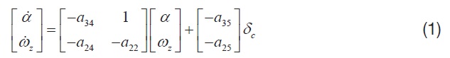
Where α― Angle of attack of interceptor; ω_z― Pitch angle rate of interceptor; a_ij―Aerodynamic force coefficients and aerodynamic moment coefficients.

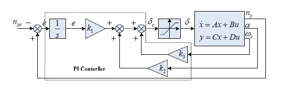
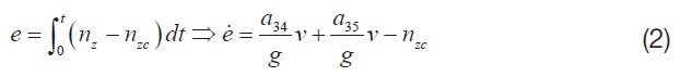
The classic three loops autopilot structure and the mathematical model are given. The autopilot structure is shown in Fig.1, in which the pitch angle rate feedback loop can upgrade the low damping of the missile; the pseudo Angle of attack feedback loop can improve the static instability of the missile and increase time response. The overload error integral variables are introduced to realize accurate tracking of the instructions [8,12]:

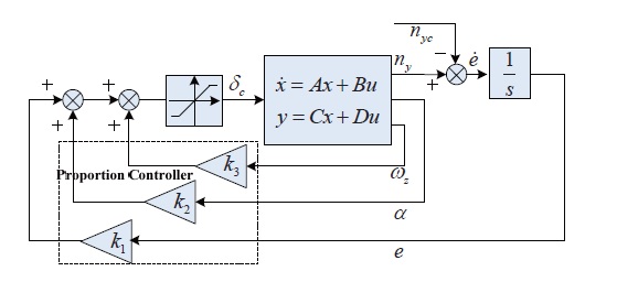
Remark1: in Fig. 1 the command of overload regarded as the input signals, the controller are proportion and integration controller; in Fig. 2 the command of overload and the integration controller regarded as the systems model, the controller is pure proportion controller. Integration Control of overload error converted into proportion control of overload error integration. The yield static output feedback control; this can resort to solving LMIs.

From the above equation (1) ~ (2), the augmented state equation is established:

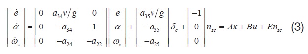
Where: v― Speed of the interceptor; g― Acceleration of gravity; n_zc― Command of the overload.

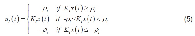
Introducing state feedback control for plant of equation (3):

Where each component of the control vector, given by u_i(t)=sat(K_ix(t)), ∀_i=1, ···, m, is defined as [5]:

The closed-loop system can be represented as:

Where A_c=A+BK, and

is a decentralized dead-zone nonlinearity.

Now, consider a matrix G∈R^m×n and define the set:

Theorem 1 [11]: for all x ∈ Σ, with ψ(kx(t)) given by (7) that

for any positive definite diagonal matrix T ∈ R^m×m.

Lemma 1[13]: The following statements are equivalent:

1. n order matrix F is stability.

2. If there exist Hermit positive definite matrices G and H, such that F=GH.

Theorem 2 [11]: If the n-order real matrix A and B are symmetric positive definite matrix, then all of the eigenvalues

of the AB are greater than zero.

The next theorem is given based on theorm1~2 and the bounded stability theory.

Theorem 3: The time-derivative of the pseudo-Lyapunov function for the linear tracking system is nonnegative, when time tends to infinity, the time-derivative of the function is null. That is to say: the maximum of the function of the tracking system is not in the initial state but in the steady state.

Proof: Choice the function as V(x)=x^TPx(P^T=P, P>0), the time-derivative of the function along the system trajectories (6) is given by

The solutions of the first-order linear time-invariant differential equations ？(t)=A_cx(t)+En_zc:

The solution for the zero initial conditions of the system is:

Taking into account (10), that:

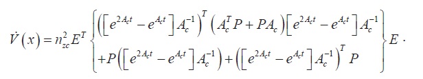
The positive and negative of

is equivalent to the positive and negative of matrix Δ:

As λ(-A_c)？0, by the lemma 1 and theorem 2, that

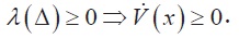
Namely, the time-derivative of the function of the linear tracking system is greater than or equal to zero,

when t → ∞.

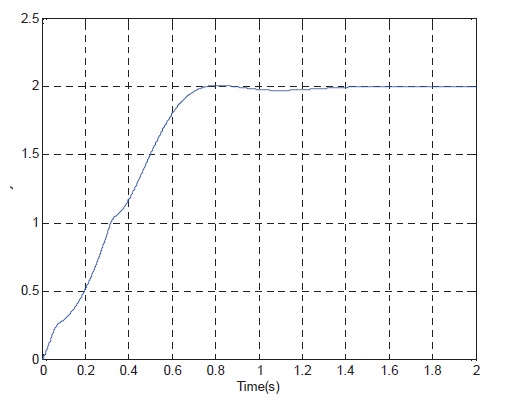
We give an example to validate that the time-derivative of the function of the linear tracking system is nonnegative to illuminate the above Theorem 3 visually.

If there exist positive definite symmetric matric W ∈ R^n×n, matrix Z∈ R^m×n and constants μ, τ, σ ∈ R, satixfy the following LMIs :

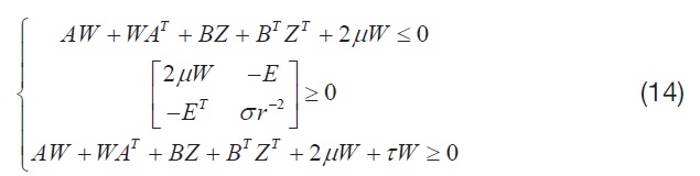
then the controller is as follows:

The eq(14) are the simplified presentation of Theorem 4 under the conditions of a linear system. The proof progress see Theorem 4, the maximum value of the system function appears in steady state, and the value is L = σ/μ, here μ is the desired closed-loop system power exponential convergence rate.

Example: given state matrix and control matrix of an aircraft at a typical flight point as follows:

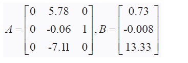
Let the negative real part of desired closed-loop pole μ=-8, and let τ=0.0001, σ=1, according to equation (14), we search for λ(W), then the following controller is obtained: K=[-24.9446 -28.2807 -0.4504].

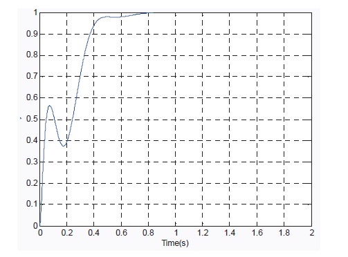
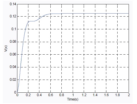
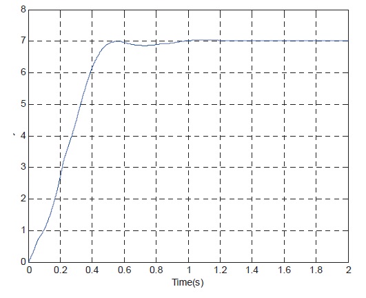
When the input command is n_zc=1, Fig. 3 shows normal overload response curve, Fig. 4 shows the function value of the tracking system varies with time.

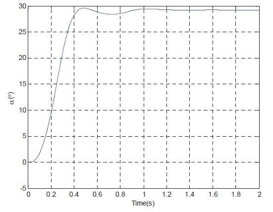
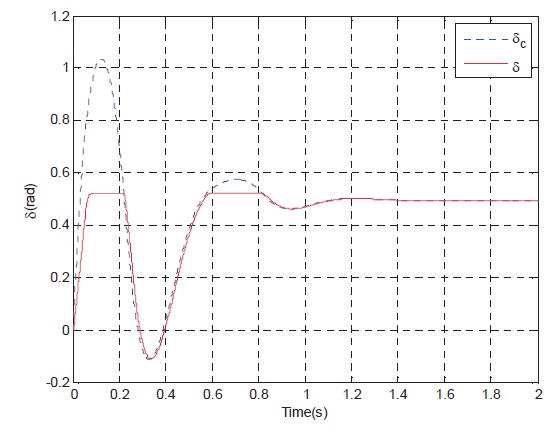
Through the simulation it is concluded that: (1) in the dynamic adjustment process, the function value for the linear tracking system increases with the simulation time, when the system states are steady, the function value reach its maximum value, just as theorem 3 said; (2) the designed control system track the instruction quickly and accurately; (3) the maximum value of the function is close to σ/μ=0.125.

Theorem 4: For any constant matrices controllable pair (A,B) with appropriate size, if there is a positive definite symmetric matrix W ∈ R^n×n, matrices Z∈R^m×n, Y∈R^m×n diagonal matrix S∈R^m×m μ, τ ∈ R, V(t)∈[1 ∞] and constant matrix κ, σ, ρ_i ∈ R, that:

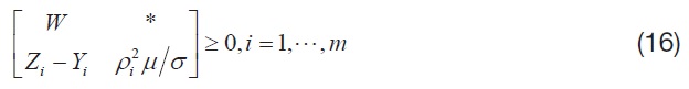
Where n_zc is overload command, ρ_i is the value of the rudder saturation and E=[-1 0 0]^T.

The controller gain is:

Closed loop system is asymptotically stable in the area of the ellipsoidal region Ξ？{x|x^TPx≤σ/μ}, and the control system input command |Kx|≤κρ.

Proof: Pre and post-multiplying (14) by diagonal matrix diag{W^-1, I}, and taking into account the variable transformations Z=KW, Y=GW, W^-1=P:

Introduction of Shur complement lemma and the (8) ensures that Ξ⊆Σ.

The response of closed-loop system converges to input command in form of power exponent through (14).

Suppose there exist τ satisfying

and taking into account (6):

By the function properties of the linear tracking system and (15):

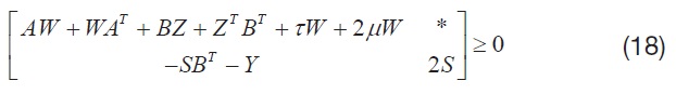
Then put (22) into (21) and applying the Schur complement lemma:

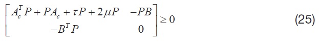
Then put (8) into (23):

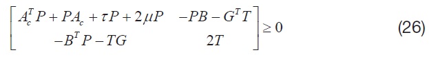
Pre and post-multiplying (23) by diagonal matrix diag{W,S}, and taking into account the variable transformations P=W^-1, S=T^-1, it follows that (16).

Suppose there exist σ satisfying the following condition:

The vector form of (25) can be rewritten as:

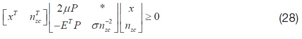
The inequality is equivalent to:

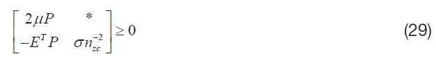
Through state transitions (27) is equivalent to (17).

According to the norm of the definition that |K_ix|≤κρ can be rewritten as:

According to the function properties of the linear tracking system, suppose there exist v(t)∈[1 ∞] satisfying the following condition:

Then:

Applying the Schur complement lemma and state transform that (30) is equivalent to (18).

We discuss now how to compute the matrices gain K from the conditions stated in theorem 4. The variables to ve found by applying theorem 4 are W, Z, Y, S, μ, τ, v, κ, σ, ρ_i ？ Since the inequalities terms involving the product between these variables, inequalities (15) ~ (18) are nonlinear matrix inequalities. To convert the non convex optimization problem into a convex optimization problem, an iterative algorithm is given as follows.

First: according to the ideal frequency response of the closed-loop system, fix the value v(t)=v₀, κ=κ₀.

Second: given the initial value μ=μ₀, τ=τ₀, the matrix inequalities of theorem 4 become LMIs. The eigenvalues of the variable W can be minimized by solving the convex optimization problem, to enhance the time response speed of the control system:

Third: Fixed W=W₀, the matrix inequalities of the theorem 4 (14) ~ (18) are converted into LMIs, The variables value of the μ, τ can be minimized by solving the following convex optimization problem with LMI constraints:

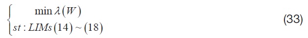
In each step, some variables are fixed and a convex optimization problem with LMI constraints is solved:

Step 0: Initialize v(t)=v₀, κ=κ₀, μ=μ₀, τ=τ₀, according to the ideal frequency response of the closed-loop system.

Step 1: solve (31) for W.

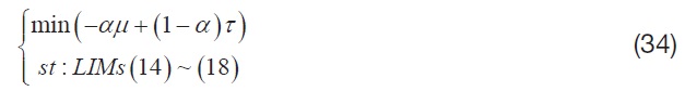
Step 2: fixed value

solve (32) for μ, τ.

Step 3: take the positive value of Δμ such that Δμ ？？ μ, Let

back to step 1 until no significant change in the optimal value of μ occurs.

The iteration between these three steps stops when a desired precision for μ is achieved.

Remark2: When v₀=1 the actuator of the control system does not appear the saturatio phenomenon, when v₀？？1 the actuator of the control ststem appear the saturation phenomenon.

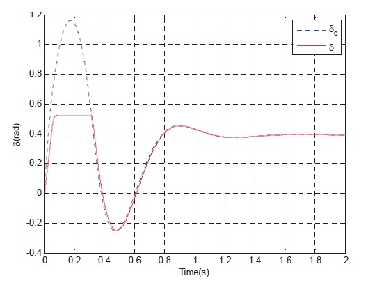
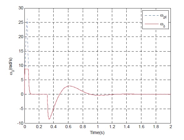
Typical flight point 1: The flight height of the interceptor is H=33 km, the speed is 3.5 Ma, Angle of attack is 20 deg, the rudder deflection angle saturation is ±30° and the rudder deflection angle rate saturation is ±500°/s. When normal acceleration command is 2g, Fig.5 show the overload response curve, Fig.6 show the Angle of attack response

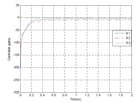
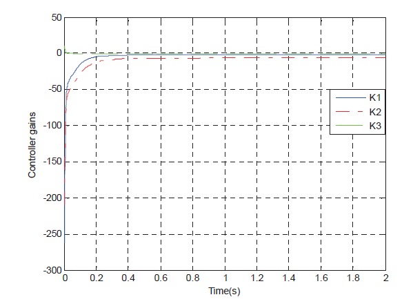
curve, Fig. 7 show the rudder angle response curve, Fig. 8 show the rudder angle rate response curve, and Fig. 9 shows the controller gains curve according to time.

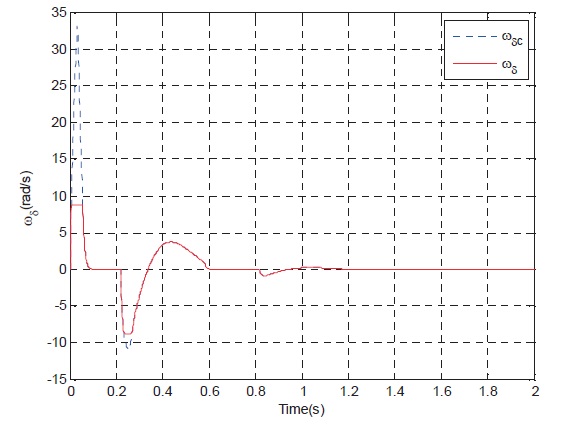
Typical flight point 2: The flight height of the interceptor is H=30 km, the speed is 4 Ma, angle of attack is 20 deg, and the rudder deflection Angle saturation is ±30° and the rudder deflection angle rate saturation is ±500°/s. When normal acceleration command is 7g, Fig. 10 show the overload response curve, Fig. 11 show the Angle of attack response curve, Fig. 12 show the rudder angle response curve, Fig. 13 show the rudder angle rate response curve, and Fig. 14 shows the controller gains curve according to time.

The simulation results of the linear control system with actuator saturation constraints show that with the increase of altitude and reduce of flight Mach, the time response speed of the control system and the ability of tracking the normal acceleration command significantly deteriorate. The Controller is a function of the input command, so fast tracking of input command can be realized.

The design control system of the near space intercept missile makes it track the command more quickly and accurately when the control input has saturation constraints. We described the classic three-loop autopilot structure and the linear tracking system mathematical model, in which Integration Control of the overload error is converted into proportion control of the overload error integration, which yields static output feedback control, this can resort to solving LMIs. We present the maximum value of the pseudo- Lyapunov function for the linear tracking system (theorem 3). This appeared at the steady states instead of the initial states based on theorem 1~2 and the Bounded stability theory. The time-derivative of the function (e.g. (10)) contains the input command, so the amplitude and frequency of the command affect the stability of nonlinear control system, designate expected closed-loop poles area for different input commands and obtain a controller which is function of input variables. The coupling between the variables and linear matrices ((15) ~ (18)) make the control system design problem non-convex. The non-convex problem is converted into a convex LMI according to the Shur complement lemma and iterative algorithm. Finally two examples of the typical flight points verify the effectiveness of the presented design technique. The proposed design method can be applied to the horizontal lateral-directional system model and arbitrary controllable system.