Due to advancements in living standards and refraction technology, refraction itself is no longer purely an ametropia problem. There is now a growing desire to construct an individual unique optometry model and integrate refraction as part of the test of visual quality. Saving time and customizing designs of refraction are now popular research, as well as application, topics.
The optical principle of refraction entails locating the conjugate focus of the retina in the focusing process. The refractive diopter can then be computed from the conjugate focus distance. Most research in this field focuses on measurement technique and the accuracy of auto-refractors or discusses subjective refraction and objective refraction [1-3]. Few studies, however, touch on the above visual technique topics from the viewpoint of the optometry model, to say nothing of using the optometry model to complement refraction services [4].
Segmenting the optical system of the eye into the cornea, aqueous, crystalline lens, vitreous, retina, and other systems and determining the sub-system parameters would allow us to use CODE V optics design software to add in emmetropia, the sub-system of a set of lens simulations known as ametropia. This would result in a new set of optical systems for the eye that would have its own refractive diopter. There would be both collective and individual factors to consider in the aforementioned process, but fortunately, the characteristics of CODE V macro programming language satisfy these requirements.
Chapter 1 of this study describes the principle and construction of the optometry model. Chapter 2 simulates the visual image produced. Chapter 3 describes the back propagation neural network (BPNN) principle. Chapter 4 describes the recognition method using invariant moments as the feature value. Chapter 5 discusses the experimental results. Finally we state the conclusions.
2.1. Construction of a Model for the Human Optical System
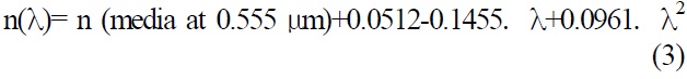
Ever since Gullstrand first proposed the optometry model in 1911, many researchers have proposed improved versions of the model [5] that would increase the eye aspheric surface and change the refractive index of crystalline lens to a variation value. The most complete and realistic proposal was the eye optometry model mentioned by Liou in 1997 [6]. The cornea and crystalline lens in the model adopted the aspheric coefficient and used a varying refractive index with relevant parameters, as shown in Table 1. The computation formula for the model’s refractive index is shown in equations (1)-(3):
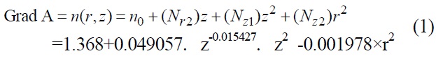
The distribution of the gradient index is represented in the form.
‘z’ is along the optical axis, ‘r’ is the radial distance perpendicular to the z axis (r2=x2+y2).
[TABLE 1.] Relevant parameters of the Liou optometry model
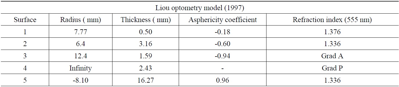
Relevant parameters of the Liou optometry model

The different ocular refractive indices at various wavelengths
This study used the Liou optometry model as a basis for constructing an original optometry model. This original model was then used to simulate the actual degree of human eye ametropia, before conducting visual image simulation by inserting macro language into CODE V.
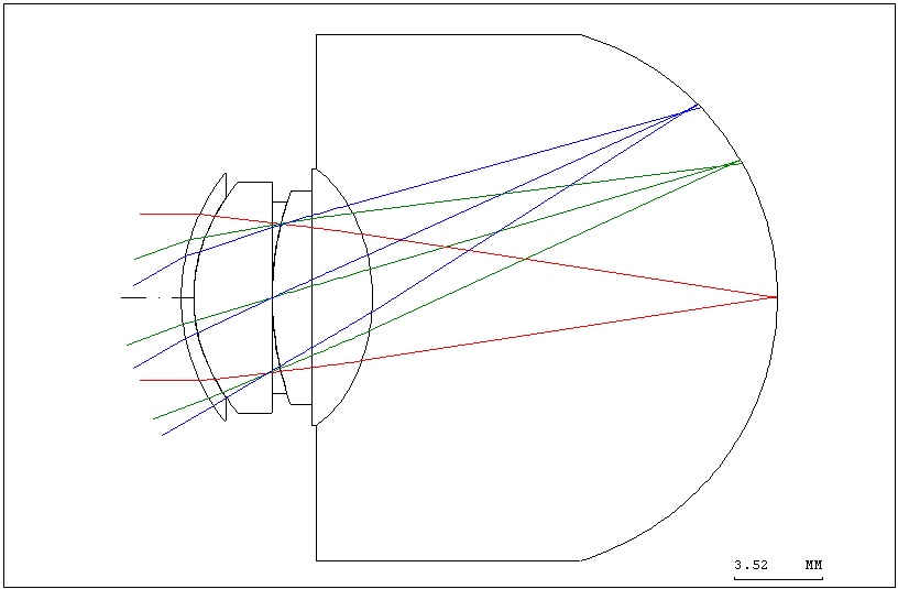
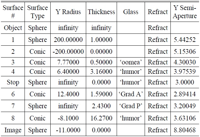
The Liou eye model built using CODE V [7] is shown in Fig. 1. The various optic parameters of the optometry model are shown in Table 2.
2.2. Simulating Ametropia in the Optometry Model
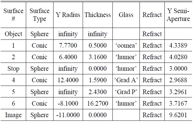
In order to simulate the ametropia of the human eye, two surfaces (one lens) were added to the corneal vertex of the original optometry model. The sphere lens (radius of curvature of 200 millimeters and -200 millimeters) simulated a myopic eyesight of 5.00D, as shown in Fig. 2. The various optic parameters of ametropia in the optometry model are shown in Table 3.
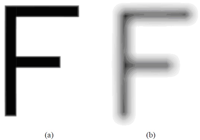
From the ametropic eye, as shown in Fig. 2, it can be seen that due to the existence of myopia, the focus on the retina becomes blurred. Therefore, the visual image produced
[TABLE 2.] The various optic parameters of the original optometry model

The various optic parameters of the original optometry model
by the human eye was also blurred due to ametropia. However, the visual images contain diffraction effects, so the location of the center of the image is relatively clear. The visual image of emmetropia is shown in Fig. 3(a), whereas the visual image of ametropia in diopters is shown in Fig. 3(b).
2.3. Back Propagation Neural Network (BPNN)
The learning process of a BPNN comprises feed-forward signal propagation and feedback signal propagation. In the process of feed-forward signal propagation, the input information is routed through hidden levels for weighting operation and, after going through transformation by Activation Function, is redirected to output level for output value operation. The neural elements in each level only affect the status at the neural elements of the next level. The operation switches to the feedback signal propagation when the output level does not meet the target value. The difference signals are fed back along the original paths to correct the weighting and bias of the neural elements at all levels. The operation
[TABLE 3.] Various optic parameters of the optometry model simulating ametropia in diopters

Various optic parameters of the optometry model simulating ametropia in diopters
stops when the differences are within the acceptable error ranges.
In the BPNN, the input of neural element j at level n denotes the non-linear function of the output of the neural elements at level n-1.

output of the k th neural element at output of n th level
f : Activation Function

sum of weighting of the output at n-1 th level

linking weighting of the neural elements between j th element at n th level and i th element at n-1 th level

bias of the j th neural element at n th level
E : error function
dk : target output value of the k th neural element
ρ : learning rate, determining the correction scale of the gradient steepest descent method
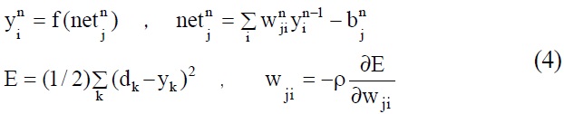
Due to the supervised learning nature of the BPNN, with the aim of reducing the difference between output and target values, the learning process of the network is to minimize the error function ‘E’. This study adopts the gradient steepest descent method to search the optimum solution on ‘E’ (the least squares of tolerances). Upon receiving an input data, the network adjusts the weighting values in proportion to the extent of sensitivity of the error function to weighting. Optimum recognition results can be achieved, through repeated computation and learning, once a minimum ‘E’ is found or a state of convergence is reached [8].
The program sequence of BPNN thermal image recognition is as follows:
Step 1: Determine the numbers of network levels and neural elements between layers.
Step 2: Set the initial weighting and bias of the network to a random number.
Step 3: Input training samples and target outputs.
Step 4: Calculate the sum of squares of tolerances between the values at the output level and the target output values.
Step 5: Calculate the difference between the output and hidden layers.
Step 6: Calculate the corrections of weighting and bias between layers.
Step 7: Update the weighting and bias between layers.
Step 8: Repeat steps 3-7 until convergence, or until the minimum is reached.
Step 9: Perform the BPNN test.
Step 9-1: Set the numbers of layers and neural elements between layers.
Step 9-2: Read the weighting and bias going through training.
Step 9-3: Input a test example.
Step 9-4: Calculate the output.
Step 10: Recall unknown or un-classified images with the accepted neural network.
3.1. Recognition of the Visual Image of Human Eye Ametropia
A total of 24 optometry models were created for eye models with myopia of diopter (-0.25D ~ -6.00D), and each model was increased by -0.25D. These would lead to corresponding visual images, with each visual image resulting in 4 visual images with different object field angles (1.5°, 2°, 2.5°, 3°) as shown in Fig. 4. The resulting visual images have different angles, though the corresponding refractive diopters are similar.
Each ametropia has 4 different direction images, which can be divided into 24 categories (numbers 1~24). Therefore, a total of 96 images were utilized, of which 48 images were provided for the BPNN for training and learning
purposes, and the remaining 48 images were utilized for testing and verification purposes. Additionally, the obtained diopter (“D”) were adopted as the output of the BPNN.
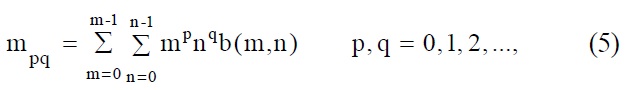
These images’ effective features were obtained as inputs to the BPNN. The BPNN was then trained to recognize objects based on the features. This study adopts the theorem of invariant moments (Hu’s moments) [9], by which normalized moments of the given image’s absolute value were taken as features, as shown in Table 4.
Some basic geometric features in a two-dimensional domain include magnitude, position, direction and shape, and most bear some relationship to moment.

the centroid of the image
m00 : the pixel is equal to 1 of total
m10 : the moment of the 'x' direction
m01 : the moment of the 'y' direction
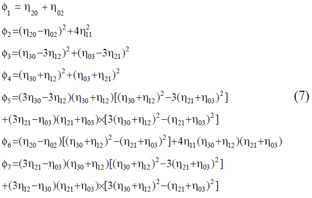
According to the invariant moments proposed by Hu’s [9], we can present the gray level value in the figure using the two-dimensional distribution matrix of b (m, n); its (p+q) order moment of the image distribution is expressed below:
The central moment (Eq. (6)), which has the property of invariance to translation, is shown below.
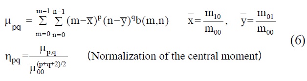
Hu derived the following seven invariant functions[10]. The seven terms listed below (Eq. (7)) were adopted in the following training and test set, as inputs to the network, instead of the actual pixel gray levels.
[TABLE 4.] Normalization of invariant moments of the 24 eye optometry model visual image files
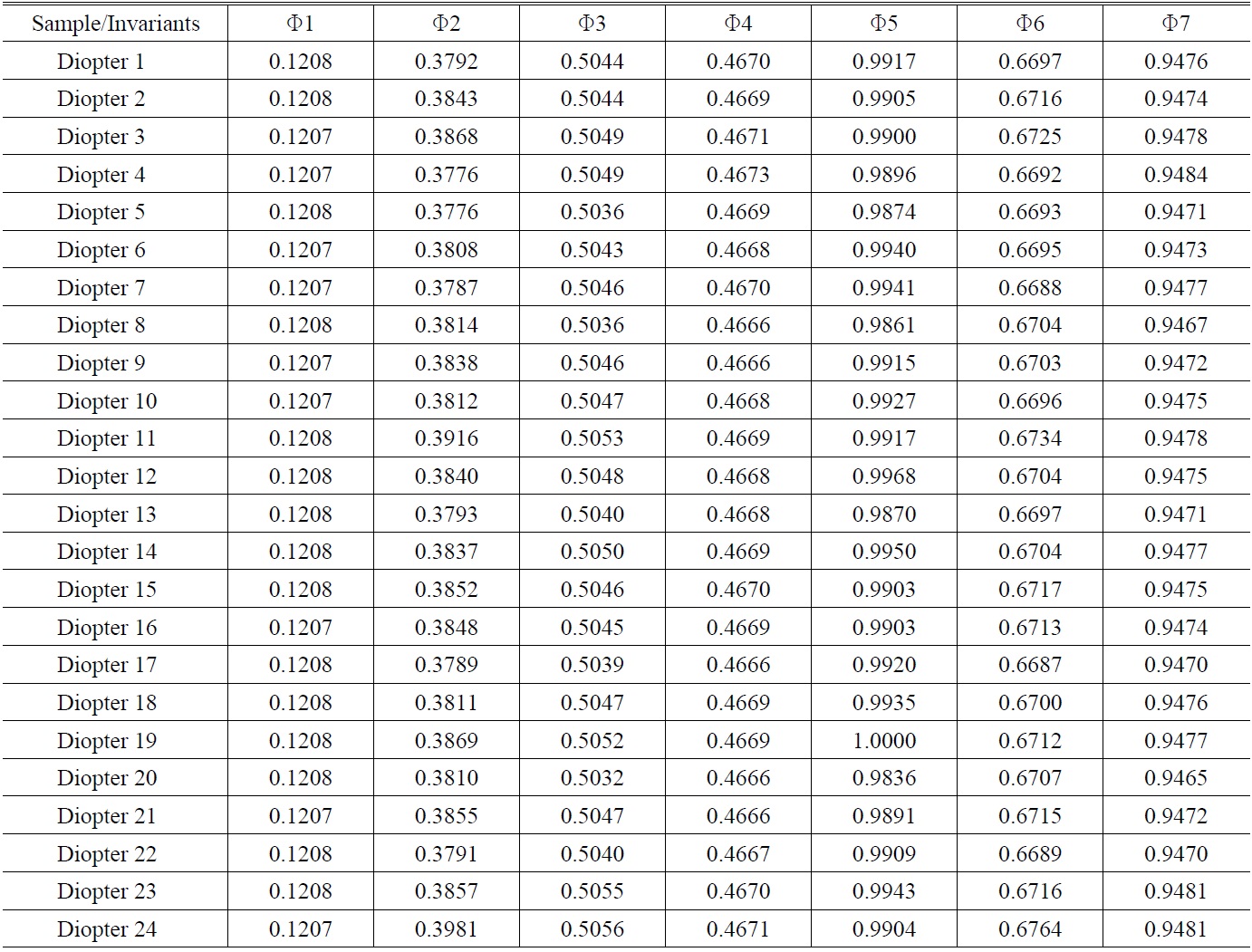
Normalization of invariant moments of the 24 eye optometry model visual image files
4.1. Discussion of Experimental Results
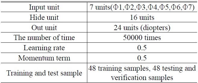
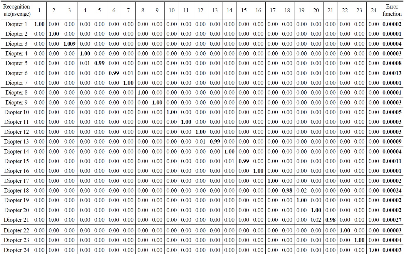
A total of 96 imaging samples at different ametropia were recognized and sorted by the BPNN. Table 5 lists the BPNN parameters associated with the 24 elements.
[TABLE 5.] Network parameters settings

Network parameters settings
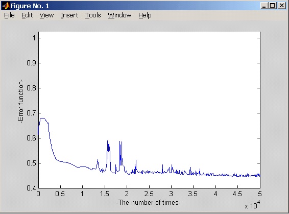
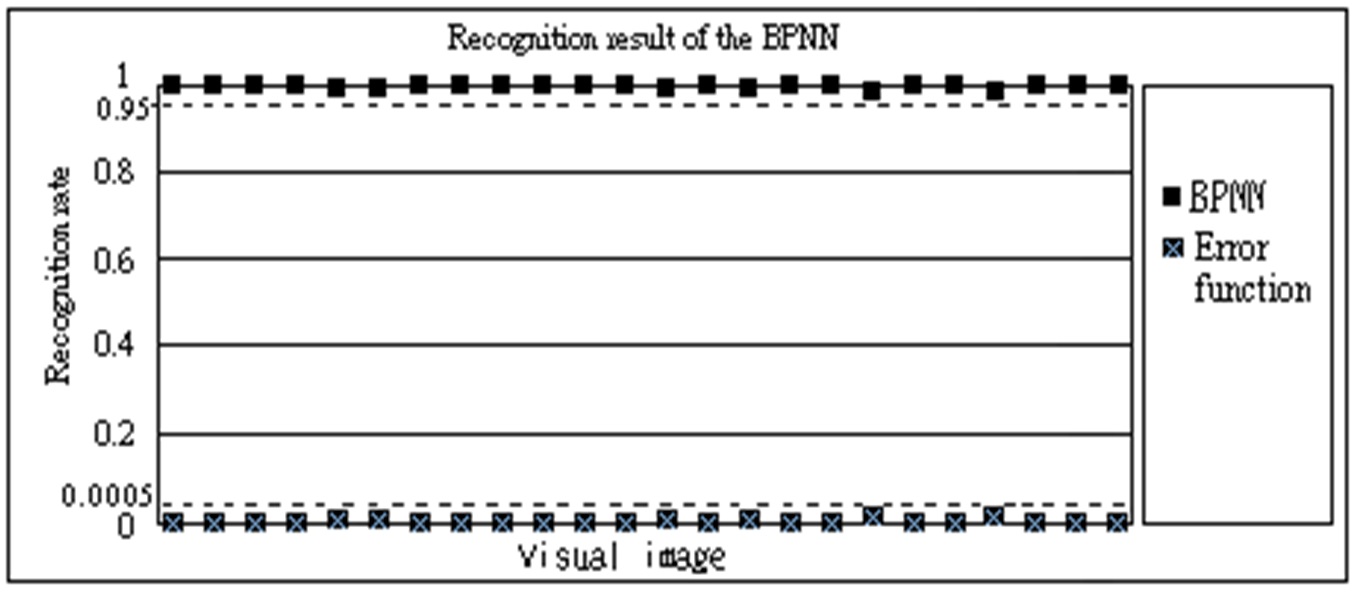
Table 6 shows the weighting and bias with convergence. Fig. 5 displays the training curve. Table 7 presents the recognition results. Results show that the accuracy achieved was above 98%, as shown in Fig. 6.
The biggest contribution of this paper was the development
[TABLE 6.] Diopter weighting and bias with network convergence
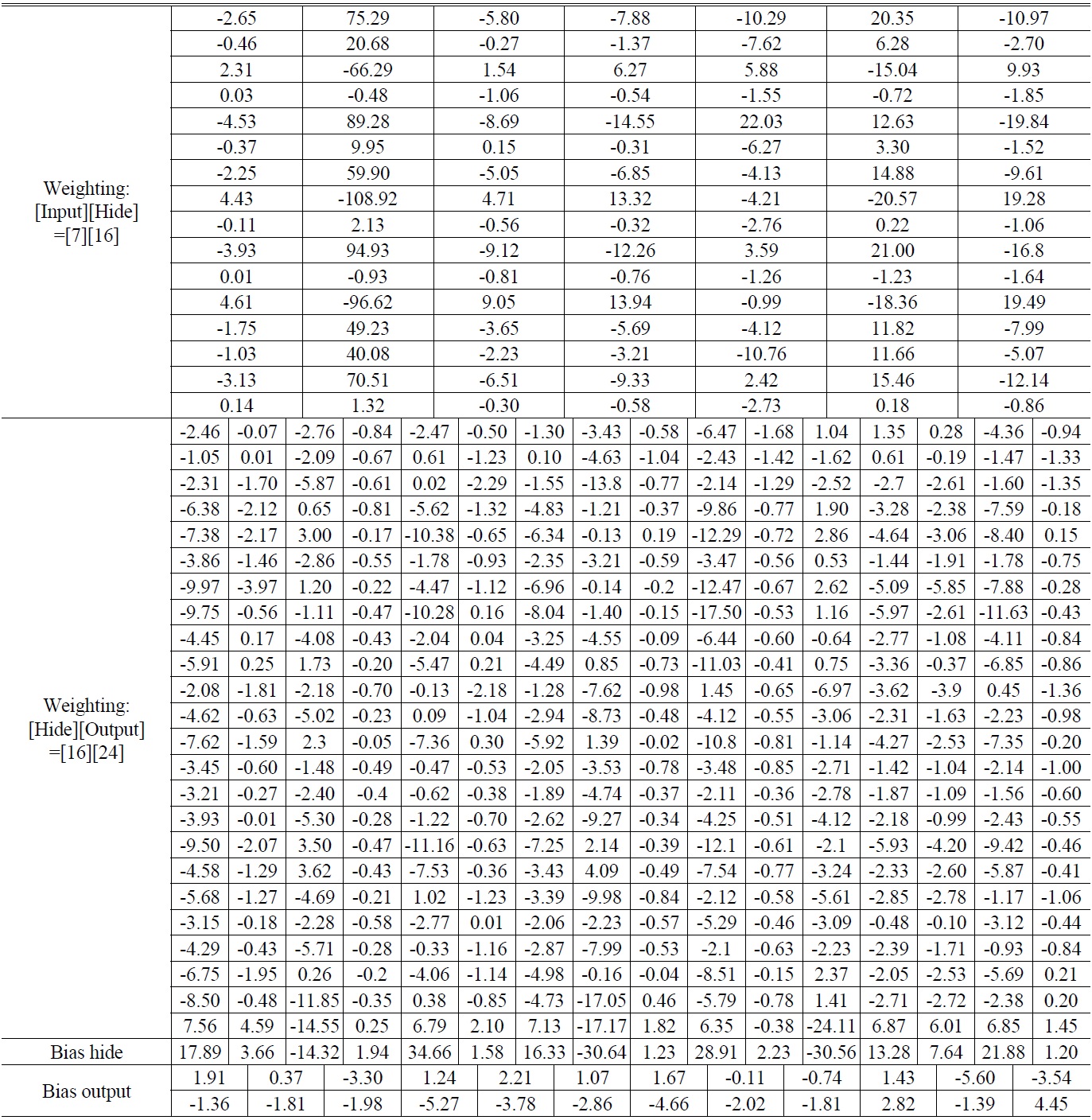
Diopter weighting and bias with network convergence
of a method that could complement the auto-refractor, taking advantage of its convenience and speed while avoiding its instability. The BPNN recognition method used could flexibly adjust the number of hide units, enhancing the speed of curve convergence through the neural network algorithm and recall capability. Together with invariant moments independent of visual images and revolving characteristics, this method could enhance the recognition of visual images to 98%, achieving results through subjective scientific methods not possible from the human eye.
Using the relevant parameters of the Liou model as a theoretical model and using the macro programming language to simulate ametropia through the Macro language effectively constructed a customized optometry model. This enhanced the efficiency of the optical design and made possible the non-spherical optical design which was complex and time consuming. The optometry model in this paper can be used to determine the refraction results and used as a personal optometry model. These computational results with scientific evidence can be applied in future medical uses or customized
[TABLE 7.] Recognition result of the network

Recognition result of the network
lenses. This paper focuses on the computation and recognition of myopia (-0.25D ~ -6.00D). Even though this approach already included the ametropia scope of most people, there is still room for improvement in the future, especially with regard to other customized designs with special needs and a high number of requirements.