The electronic semi-conductor device industry has rapidly developed and become focused on minimization in recent years. Super minimal semi-conductors with high performance are frequently used for memory chips with large capacity. On occasion, these memory chips, which can contain information, have been used illegally. Accordingly, detection of hidden devices becomes difficult because of complex hiding method. Detection of a tiny chip made by the semi-conductor or the false junction material composed of a semi-conductor and a metal has been made possible by the development of a nonlinear junction detector (NLJD) [1-3].
The performance of NLJD System depends particularly on the antenna characteristics because the antenna has to satisfy broad bandwidth including transmitting frequency (Tx) and receiving frequency (Rx) band. Additionally, in order to minimize the effect of power reduction by coupled wave from the hidden device, the high gain circular polarization antenna has been mainly used for NLJD system application [4-6]. In this paper authors designed the high gain spiral antenna with novel Archimedean spiral slit on ground plane to realize the circular polarization and designed the new cavity [7] added conical wall to realize the high gain. The gain and axial ratio of spiral antenna proposed by reference [4] had been decreased due to multi resonance characteristics. In order to solve an above problem, authors have proposed the novel spiral antenna structure that it was composed of the extended conical wall with the conventional circular cavity wall and the optimized archimedean slit conductor on the ground plane by current distribution. The resulting antenna showed a gain of 9.5 dBi higher than the conventional gain specification of 6 dBi at the interested bands.
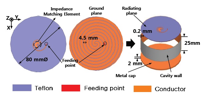
Fig. 1 shows an antenna configuration with a conventional 4.5-turn spiral slit structure on the ground plane [4]. A diameter of the spiral antenna is 80 mm
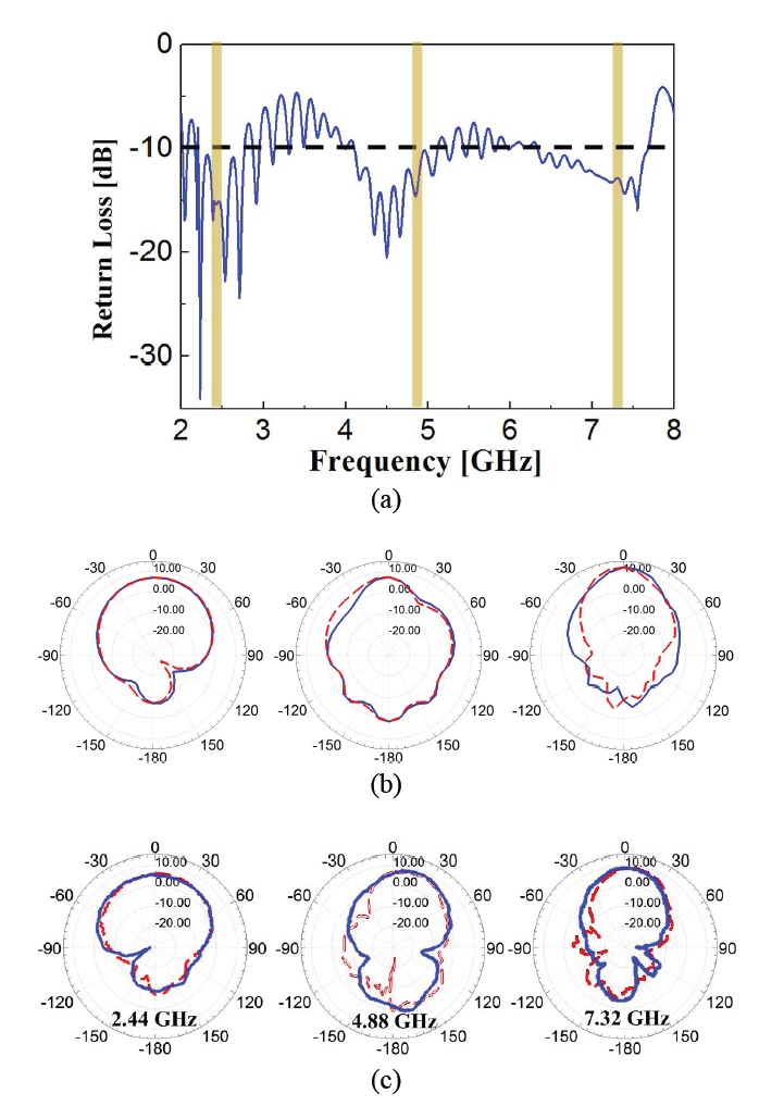
Fig. 2(a) shows the simulated return loss of antenna structure shown in Fig. 1. The return loss is ?10 dB lower at the interested 3 bands. Fig. 2(b) and (c) show the simulated and measured gain radiation pattern of the antenna structure shown in Fig. 1.
Table 1 shows the simulated gain at the interested center frequency, where
[Table 1.] Simulated gain of antenna structure in Fig. 1
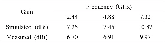
Simulated gain of antenna structure in Fig. 1
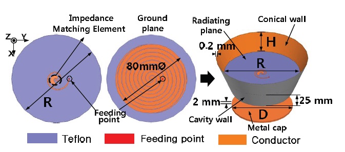
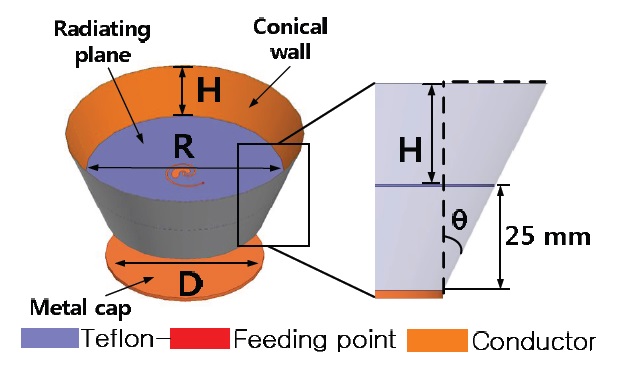
In order to increase gain of conventional antenna structure in Fig. 1, authors proposed the improved cavity wall with the added conical wall as shown in Fig. 3. In addition, an optimum conical wall was designed by studying the parameters of conical’s radius (
Fig. 3 shows the spiral antenna composed of a conical wall structure. The diameter of the Archimedean spiral slit on the ground plane is 80 mm
The symbol
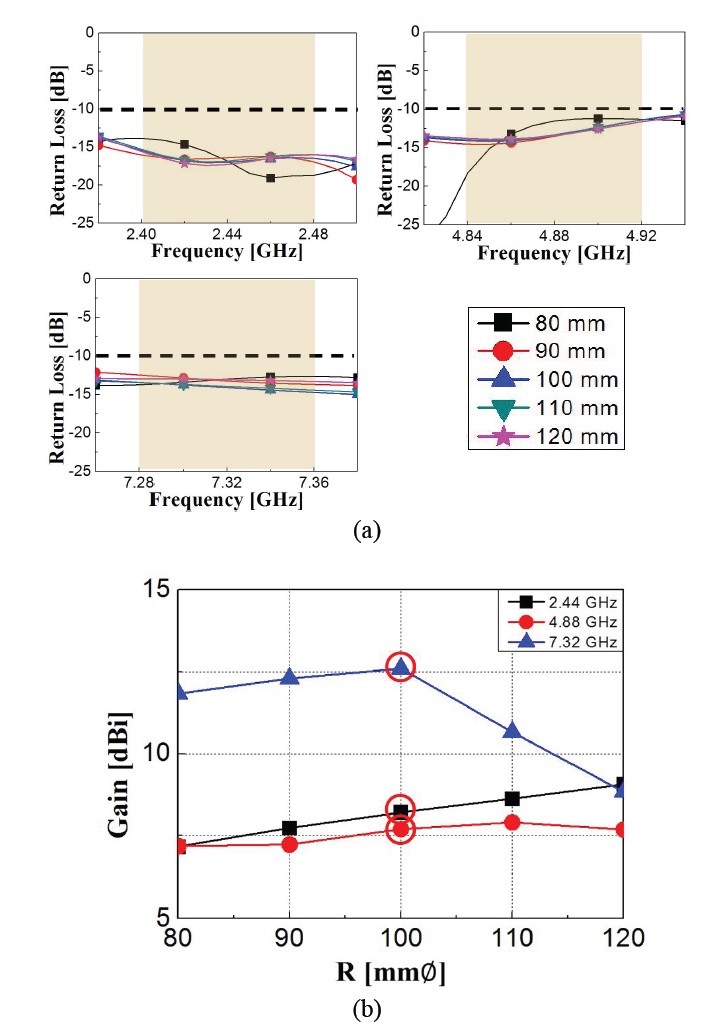
The simulated return loss shown in Fig. 4(a) is still ?10 dB lower at the interested 3 bands. In Fig. 4(b), the simulated gains of the transmitting and the 2nd harmonic frequency are increased with the increase of R. However, the gain simulated at 7.32 GHz of the 3rd harmonic frequency shows the maximum value of 12.5 dBi, when
Fig. 5 shows the spiral antenna cross-section composed of a conical wall structure. When
Thus, the optimum parameter value of
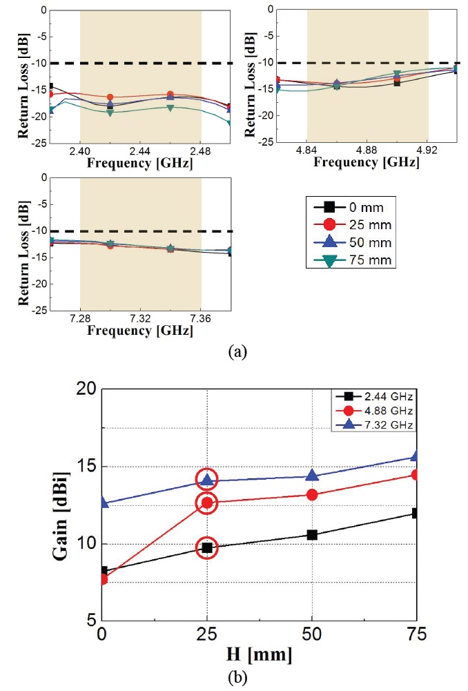
Fig. 6(a) and (b) show the simulated return loss and gain characteristics by variation of the conical wall height from the radiating plane. The values of
The return loss is still ?10 dB lower at the interested 3 bands, even though H is changed. Fig. 6(b) shows the simulated gain by variation of
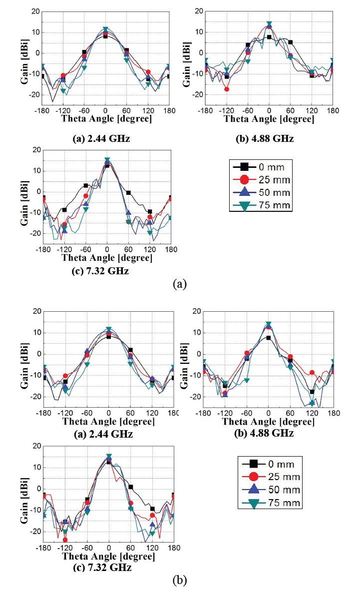
Fig. 7 shows the simulated radiation pattern by variation of H. The difference in the beam width with a conical wall height is not very critical, so that even though gain depends on
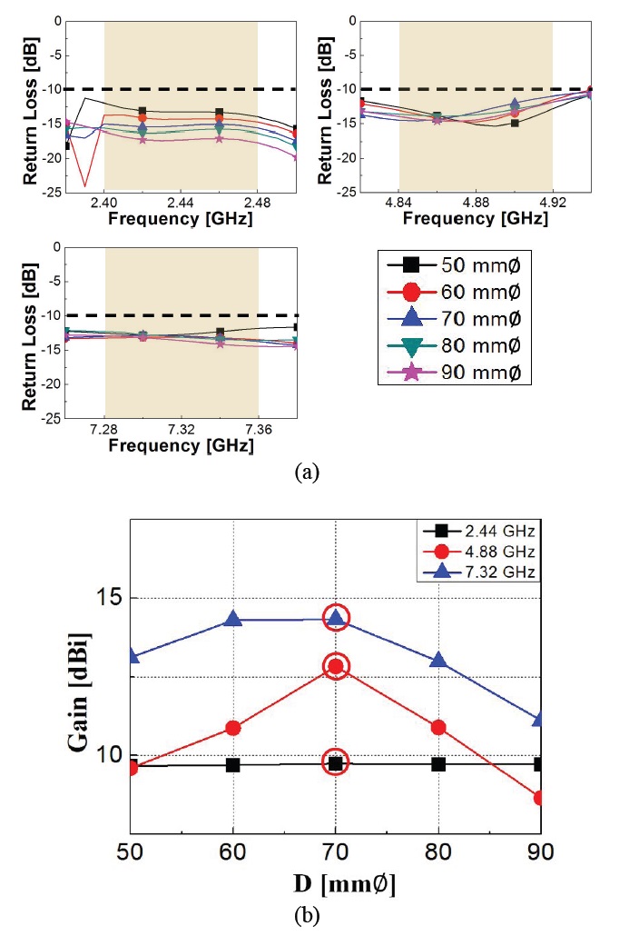
Fig. 8(a) shows the simulated return loss characteristics by variation of the metal cap diameter
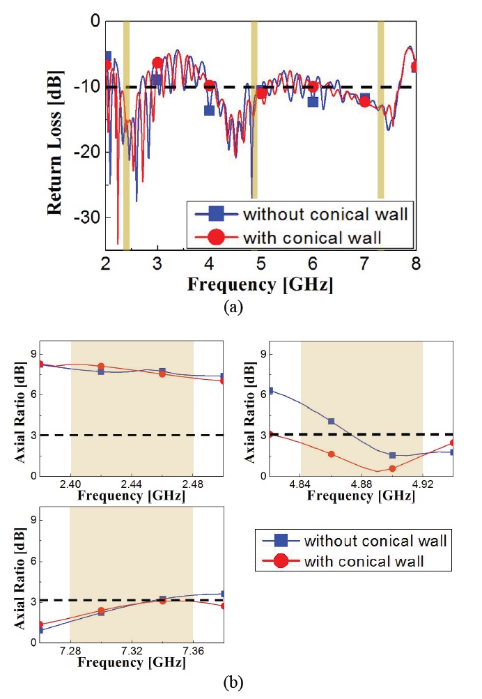
Fig. 9 shows the simulated results and with and without a conical wall for 4.5-turn spiral slit on the ground plane. The simulated optimum parameter values of
However, even though the gain is markedly improved by the added conical wall, the axial ratio at the Tx band remains poor, at an average of 7.5 dB as shown in Fig. 9(b). This is caused by the current reflected from the metal cap. The solution to the poor axial ratio problem was sought by examining the current distribution of archimedean slit on the ground plane at 2.44 GHz.
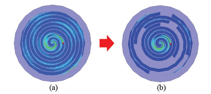
Fig. 10 shows the comparison of the electric current distribution of the archimedean slit structure located on the ground plane at 2.44 GHz [5]. The electric current of the conventional 4.5-turn spiral slit structure on the ground plane appears somewhat stronger than the current for the optimized slit structure in Fig. 10(b). However, this is due to the sum of the current with the circular polarization that is radiated in the opposite direction by current reflected from metal cap, as shown in Fig. 1.
The reason for the current generation with reverse polarization is that the quarter wavelength of 2.44 GHz is longer than the 25 mm cavity wall height. The conventional 4.5-turn spiral slit on the ground plane is newly designed, as shown in Fig. 10(b), and proposed in [5]. The gain of the optimized slit shown in Fig. 10(b) was almost unchanged when compared with the conventional antenna in Fig. 1 [5]. This means that the spiral slit structure on the ground plane was optimized by controlling the electric current distribution at 2.44 GHz, and the gain value was constantly maintained even though the physical conductor surface size was reduced by removal of the slit.
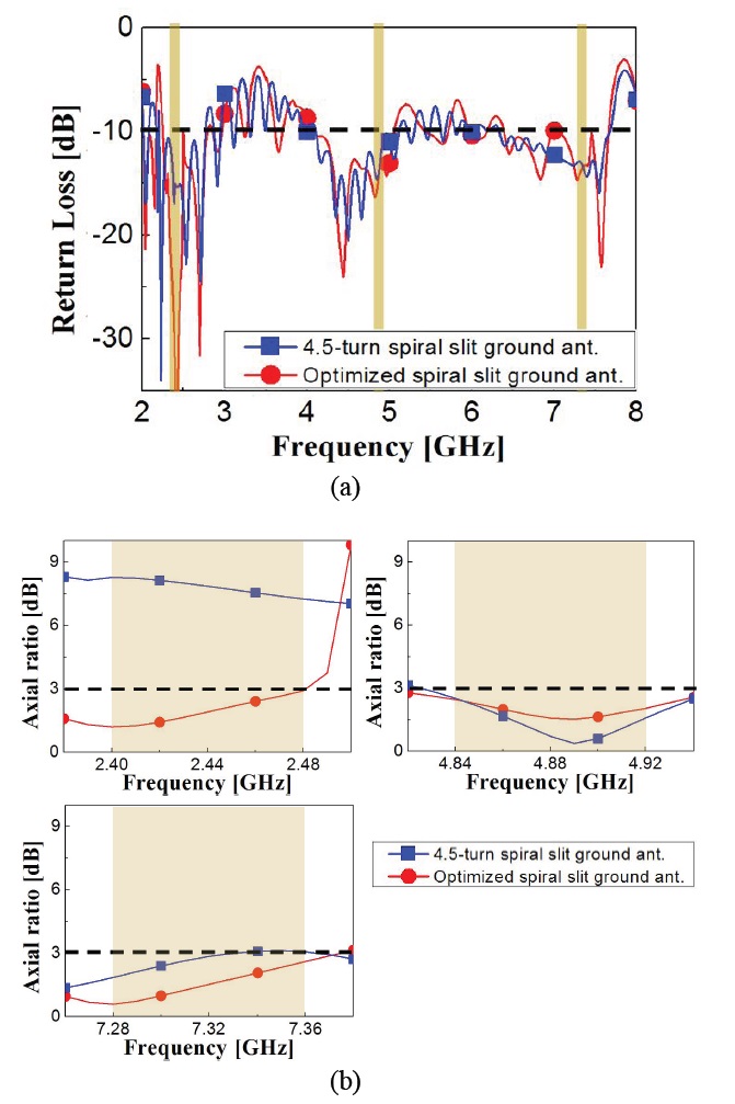
Fig. 11 shows the simulated return loss characteristics of the antenna with respect to two kinds of archimedean slits on the ground plane as shown in Fig. 10(a) and (b). The simulated return loss of the 4.5-turn and the optimized spiral slit with the conical wall shows very similar results, and it is maintained ?10 dB lower at the interested 3 bands. This means that the return loss is independent of the spiral slit structure on the ground plane. On the other hand, the axial ratio strongly depends on the spiral slit structure, as shown in Fig. 11(b). The simulated axial ratio at 2.44 GHz, as well as at 4.88 and 7.32 GHz, is clearly improved by the optimization of the spiral slit structure on the ground plane. The axial ratio is 3 dB lower at the interested 3 bands.
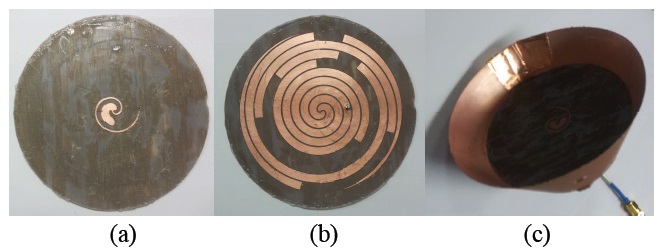
The effectiveness of the proposed antenna was verified by fabricating the novel antenna with an optimized slit on the ground plane and with the added conical wall, as shown in Fig. 12.
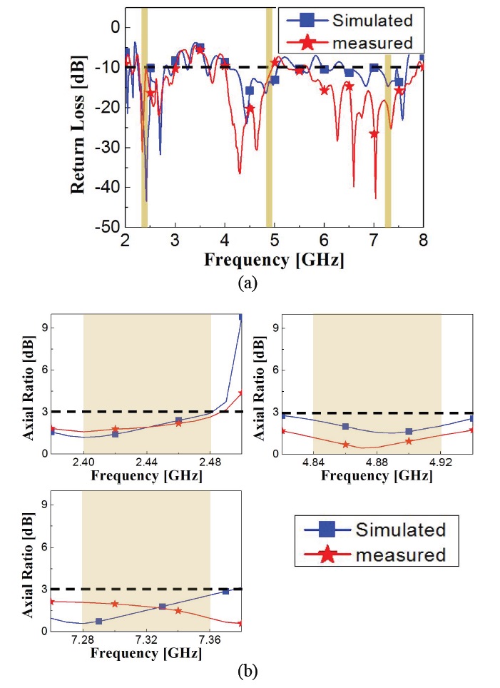
Fig. 13(a) shows the comparison between the simulated and the measured return loss of the designed and fabricated antenna, respectively. The measured return loss shows reasonable agreement with the simulated one, even though it is slightly different. Fig. 13(b) shows the comparison of the simulated and the measured axial ratio. The simulated axial ratio and the measured axial ratio show good agreement and the ratio is maintained at 3 dB lower at the interested band.
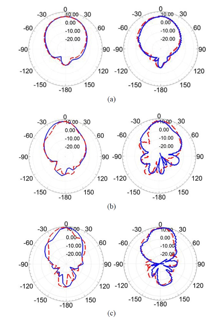
Fig. 14 shows the comparison between the simulated and the measured 2-D gain patterns at 2.44, 4.88, and 7.32 GHz.
The solid and dotted lines indicate the main E-field polarization of the X-Z plane and of the Y-Z plane, respectively. The measured E-field gain patterns showed very fine agreement with the simulation results, as shown in Fig. 14.
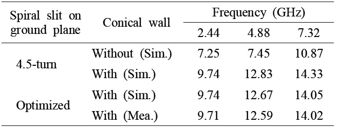
Table 2 shows the gain comparison of the spiral antenna with the conventional 4.5-turn spiral slit and the newly designed optimized slit on ground plane, with and without the conical wall antenna. As seen in Fig 8(b), the gain is controlled by with and without conical wall.
[Table 2.] Gain comparison of the spiral antenna (unit: dBi)

Gain comparison of the spiral antenna (unit: dBi)
[Table 3.] Axial ratio comparison of the spiral antenna (unit: dB)
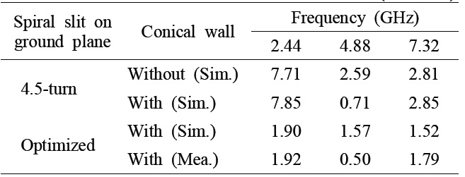
Axial ratio comparison of the spiral antenna (unit: dB)
For example, the gain of the spiral antenna with the conical wall and with the 4.5-turn spiral slit on the ground plane is almost the same value when compared with the optimized slit antenna gain as shown in Table 2. This means that antenna gain has no relation with slit structure.
Table 3 shows the axial ratio comparison of the spiral antenna. As in Fig 9(b), the axial ratio is improved by the newly designed slit on the ground plane. It is not dependent on conical wall. The quarter wavelength of 2.44 GHz is longer than the height of the cavity wall in Fig. 1; therefore, the axial ratio becomes increasingly worse due to the current with the opposite circular polarization reflected from metal cap. The improvement of the axial ratio is realized by the novel design of the slit on the ground plane.
This paper proposed a design for a spiral antenna with a conical wall to obtain a high gain. One application of the proposed antenna is the NLJD system. The gain and the axial ratio of spiral antenna were improved by using a conical wall and a newly designed Archimedean slit on the ground plane for a conventional antenna with a circular cavity wall and a conventional 4.5-turn slit. The improved gain of 9.5 dBi above at 2.44 GHz and the good axial ratio of 1.9 dB lower at the interested band are realized by the added conical wall and the newly designed slit from current distribution control on ground plane, respectively. The measured return loss was ?10 dB lower at the interested band. The simulated return loss and axial ratio of proposed antenna agreed well with the measured results. The measured E-field gain patterns of the X-Z plane as well as the Y-Z plane also showed very good agreement with the simulated results.