Unlike the case of LNG cargo containment system in the seagoing LNG carriers, the design of the structurally reliable cargo containment system for the offshore LNG units such as LNG FPSO or FSRU is far more challenging task due to the unprecedentedly large size of the storage tank and harsh environment that the structure is exposed to. Also, the operation of the offshore LNG units has to be made without filling limitation, which is not the case of seagoing LNG carriers, and this is one of the reasons why care has to be taken in the design of the cargo containment system of offshore LNG units. The above mentioned aspects of offshore LNG units, which is different from the seagoing LNG carriers, tends to prohibit the designers from relying on the past track record of LNG carriers in the design of cargo containment system of offshore LNG units. It is very well known that the liquid motion inside cargo tank under high and low filling case of LNG carriers is totally different from that under partial filling case, for example, the filling level around 30~40% of tank height.

The difficulties entangled with the design of structurally reliable cargo containment system arise due to, fundamentally, the randomness of sloshing phenomenon. The liquid motion inside cargo tank is totally chaotic so that statistical approach is necessarily required to derive design sloshing impact load. And this aspect forces the designer to idealize the sloshing impact pressure with limited number of parameters, for example 2 or 3, which are able to well capture the characteristics of the pressure time history. This idealization process sometimes misses very important features of the pressure time history, such as rising pattern and decay rate etc., leading to the situation that the robustness of the strength assessment is questioned.

Common practice of the strength assessment of the membrane type cargo containment system usually starts from the impact idealization with 2 parameters, i.e., the peak pressure and rise time. Sometimes, the area under pressure time history is taken as a parameter, but this impulse is of little relevance to the structural dynamic response because the response of the cargo containnment system under impact load is the matter of dynamics and the impulse itself is the quantity without temporal characteristics. The amplification of the structural response when the dynamic load is applied peaks when half of the natural period of the structure matches with the rise time of the load. In line with this, the decay time is also one of the important factors influencing the dynamic behavior of the underlying structure, but it is often not considered explicitly due to the complexity that comes into effect during the statistical postprocessing stage.

Sloshing phenomena in LNG cargo containment system gathered a lot of research interests and there have been many attempts to develop a reliable methodology through which the sloshing design load can be derived with confidence. Due to the randomness of the sloshing impact pressure, researchers focused on the long-term prediction of the sloshing impact load measured from the scaled model tank (Gavory and de Seze, 2009; Pastoor et al., 2005; Rognebakke et al., 2009; Fillon et al., 2011; Kuo et al., 2009). Recently, Graczyk and Moan (2008) investigated a large sample of sloshing pressure measurements and intensively studies the magnitude of individual sloshing impact events and their temporal and spatial patterns. They found that the duration of these impacts are the order of the natural frequency of underlying insulation structure so that the details of the time history is very important in deriving the design sloshing impact load. They also found that the magnitude of the sloshing impacts is larger with longer duration, smaller ratios of rise time to duration and larger spatial extents especially when the filling level is low. Kim et al. (2010) carried out extensive study on the strength assessment of the membrane type cargo containment system of LNG-FPSO with two-row tank arrangement. The long term design sloshing load was extracted from the model test and insulation structure with different reinforcement level, exposed to the sloshing loads was analyzed by transient finite element analysis.

Turning to the more practical design aspect, a lot of research efforts have been made to develop the reliable strength assessment procedure of the cargo containment system under sloshing impact pressure by the classification societies such as ABS (2006), BV (2009), DNV (2006) and LR (2009). Majority of the procedures developed by the classification societies are based on the so called load-based approach, where the design sloshing impact pressure is extracted out of the pressure time history after some temporal idealization and parameterization. Normally, a single impact event is modeled with a triangular shape which can be represented by two parameters, i.e., rise time and peak pressure and the separate statistical analysis is performed for both parameters to derive design sloshing load. It is pointed out by DNV (2006) and LR (2009) that the time history of the pressure impulse is usually very complex and it is not always clear how to idealize the pressure pulse. It also is pointed out by ABS (2006) and BV (2009) that it would be more correct to calculate the statistics of structural response instead of using the statistical values based on the pressure peaks. Kim and Kim (2007) proposed response based strength assessment procedure. They took advantage of the convolution integral method, which is popularly used in the response analysis of a linear system under arbitrary excitation, in the structural response calculation of the cargo containment system. The stresses developed in the structure is calculated by impulse response function method and the pressure time history is converted into stress time history without relying on the time consuming transient dynamic finite element analysis. Then, the stress peaks are extracted out of the stress time history and the statistically meaningful stress level is extracted from the long duration time history of the converted stress signal. Nho et al. (2012) applied the methodology to the strength assessment of Mark-III cargo containment system. They analyzed the structural response of the cargo containment system under given time history of the sloshing impact pressure which was obtained through the small scale model test and derived the failure pressures with respect to the duration and skewness of the impact.

The present study is motivated by the achievement of the research of Kim and Kim (2007), targeting the improvement of the numerical efficiency of the response based strength assessment method. To achieve the goal, the sloshing pressure time history is decomposed into wavelet basis function, instead of triangular impulse used by Kim and Kim (2007), to minimize the number of basis function, which is the key factor to improve the numerical efficiency. After the signal decomposition, the response of the structure is calculated by finite element method under each wavelet basis of different scale. Then the response of the structure throughout entire time span is obtained by convoluting the wavelet transformation coefficients with the wavelet response function of different scale. Finally, the statistical value, i.e. 3 hrs maximum stress level, is derived through 3-parameter Weibull fitting on the extracted stress peaks out of the converted stress time history. The results are cross compared with traditionally used load based approach where temporal idealization of impact event is used.

The current practice of the strength assessment of cargo containment system under sloshing load is mainly proposed by the ship classification society and Gastransport & technigaz (GTT), the patent holder of the membrane type LNG cargo containment system. Due to the complex nature of the sloshing phenomenon inside cargo tank of a floating structure, there still seems to be a lot of uncertainties related to both hydrodynamic and structural mechanics point of view. Some of main uncertainties relevant to the design can be listed as below,

Pressure time trace.

Pressure traveling.

Scale law.

Hydroelasticity effect.

Material behavior under cryogenic condition.

Material behavior under fast dynamic load.

There probably may be many others except for those listed above, but these are main uncertainties that are targeted to be overcome by many researchers. First three items are more or less hydrodynamics related issues and the final two about material behavior are more relevant to the structural mechanics, with hydroelasticity effect is somewhere in between. It may be fair to say that the different priority should be assigned to the each item and should be tackled with different weight. The present study is related only to the uncertainty related to the very first item, i.e. pressure time trace.

Usually, the sloshing impact pressure is idealized as a triangular shaped impulse load with the three parameters that characterize the shape, i.e., rise time, peak magnitude and decay time. These three parameters are of prime importance from the structural response point view both in terms of the time and the magnitude. It is needless to say that the pressure magnitude is directly related to the structural response, but the other two temporal parameters are also very important since it has direct impact on the occurrence of the resonant behavior between the structure and the excitation in dynamic condition. Normally, when the rise time of the impact load acting on the structure stays near the half of the natural period of the structure that is exposed to the

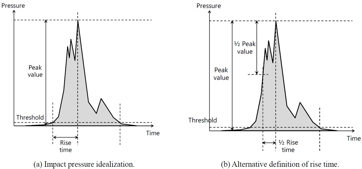
impact load, one can expect the structural response tends to be magnified by amount of, so called, dynamic amplification factor. The decay time is also closely related to the dynamic behavior of the structure since it is the control parameter of the attenuation of the structural response. However, to simplify the statistical analysis procedure, it is often assumed that the rise time equals to the decay time so that only two parameters remain to model the idealized triangular shape. Fig. 1 shows two methods, proposed by DNV (2006) through which a single impact event is idealized by the two parameters. First of all, the threshold value is empirically chosen and the time that takes for the pressure to reach the peak value from the threshold value is defined as the rise time. There is an alternative way to define the rise time as shown in Fig. 1(b). In this alternative definition, the half of the rise time is defined as the time between the pressure peak point and its half. The rise time matters when it comes to the structural response under dynamic load since the rise time, which is the time for the load to reach its peak value, is the key factor to determine whether the excitation is in near resonance with the structure or not. Therefore, once there is some obscurity in the definition of the rise time linked with the pressure peak during the triangularization, it is very likely that one may miss the important dynamic nature of the structural response calculation.

Fig. 2 shows typical schematic view of the pressure time history when gas is entrapped by the surrounding liquid impacting the corner of the tank. This is one of typically observed phenomena near the upper ceiling of the tank when the filling level is relatively high. The oscillation frequency depends on the compressibility of the trapped gas together with its volume and shape, and it holds the possibility that the oscillation causes the resonance with underlying structure depending on the local natural frequency of the structure that is exposed to the oscillating pressure load. Also the dynamics behavior of the structure may differ between the two stages, i.e. the steady rising stage during the early phase of the impact and the oscillating stage near the top of the hump. In this regard, the definition of single rise time for this impact event becomes questionable. Moreover, Fig. 2(b) clearly demonstrates that there may be two different choices of rise time, case 1 and case 2, depending on the selection of the pressure peak. If one strictly follows the idealization given in Fig. 1, it is clear that the real dynamic nature of the impact pressure during the steady rising stage is lost, not to speak of being unable to consider the dynamic nature of the impact pressure during the oscillation stage. Sometimes the situation may become really complicated due to the interaction effect of the acting pressure.

To check the effect of the pressure impact idealization with simple triangular shape of equal rise and decay time, a simple numerical test has been carried out using an example of sloshing impact pressure applied on the cargo containment system model. Fig. 3(a) shows a single impact event which was chosen from the model test of 1/50 scale. The impact pressure peaks around 0.025 sec in the small boxed graph shown in upper right corner and this peak is magnified in the main window. The impact pressure is modeled with simple triangle shape and both pressure peak magnitude and corresponding rise time are defined following the definition shown in Fig. 1. Fig. 3(b) shows the finite element model of the GTT NO96, a type of membrane insulation system developed by GTT, non-reinforced insulation box. The half of the box is modeled using 4-node quadrilateral shell element considering the symmetry and the symmetric boundary condition is applied on that plane. The bottom of the insulation box is supported by the resin ropes and these are modeled with 8-node hexahedral solid element. The bottom of the resin ropes is fully fixed. The pressure shown in Fig. 3(a) is applied on the top surface of the box and the stress time history at location A is monitored. The explicit transient dynamic analysis has been carried out using the commercial finite element program ABAQUS Ver.6.8. The material properties for the plywood and the resin are given in DNV (2006).

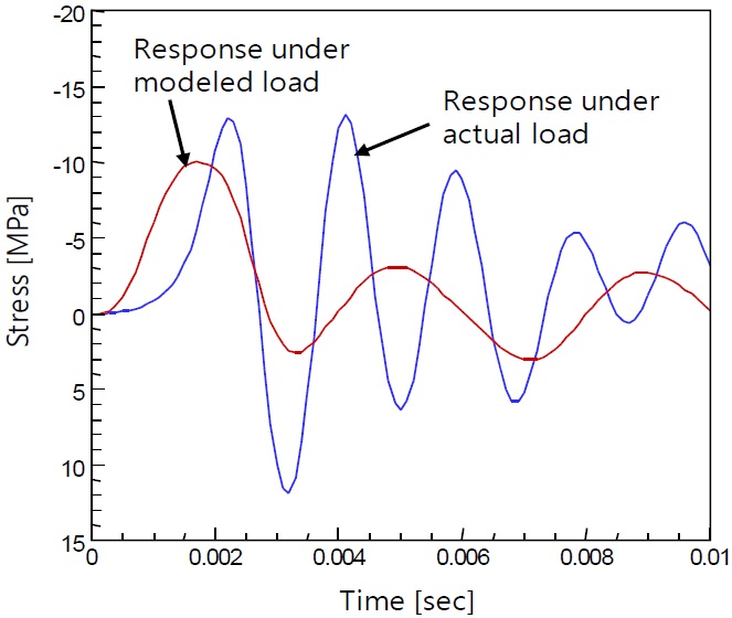
Fig. 4 shows the comparison of the time history of the vertical component stress at the location A. As can be seen in this graph, the modeled load predicts somewhat lower stress value compared to the stress under the actual load. This difference between the two cases may be ascribed to the different load rising pattern during the early stage of the pressure signal, shown in Fig. 3(a). The modeled load misses the smoothly rising pattern in the early stage of the pressure action that the actual load follows and this small difference between the two cases results in the stress deviation shown in Fig. 4. Based on this, one may conclude that the small difference between the actual load and modeled load may induce somewhat large difference in the response of the structure.

It is well known that the sloshing phenomenon is strongly nonlinear and this is why a lot of research efforts are devoted to the sloshing problem without achieving some practically fruitful output. The strong nonlinear characteristics of the sloshing phenomenon forces the researchers to rely on the either nonlinear computational fluid dynamics (CFD) or the model test for the sloshing load evaluation, though the former one is still in not practically useful stage. As to the response of the structure part, the situation is not as difficult as the hydrodynamic part, but the problem is that it is not readily achievable to obtain the crystal clear sloshing design load both in terms of pressure magnitude and its temporal characteristics. The response based approach, rather than load based one, may play some role in solving this issue thanks to its clarity from statistical analysis point of view. Given this condition, the breakthrough, at least from temporal characteristics of the sloshing impact pressure, can be made once the stress time history can be obtained in appropriate way from the sloshing impact time history. This is the key to the success of response based approach.

The main idea to obtain the structural response with rapidity comes from the fact that the structural system is linear. Once the system is linear, the output can be obtained by synthesizing the response component which corresponds to the input component. This can be done either in time and frequency domain by using convolution integral and Fourier transform respectively. Due to the presence of the sharp peaks and discontinuity, Fourier transform does not seem to be the right way to follow. The convolution integral using impulse response function may be the potential candidate, but the second thought should be given to it in terms of the numerical efficiency. In the convolution integral method using the triangular impulse, the interval of the impulse has to be small enough to capture the sharp peak, and this interval should be the order of the sampling frequency. This triangular impulse with very short interval definitely deteriorates the numerical efficiency once it starts to sweep the region where the signal varies rather slowly, in which case the interval may be increased. Considering the drawbacks of the above mentioned two approaches, the best way seems to be the one which can overcome the inefficiencies that the two approaches have. Therefore, the new method has to be able to capture the sharp peaks or local discontinuities with small number of basis and also has to be able to reproduce slowly varying signal without using too many basis. The ‘Wavelet’ is the right choice for that.

It is well known that the wavelet transforms have some advantages for representing the signals with sharp peaks and discontinuities. Standard Fourier transform decomposes the entire signal with trigonometric functions. It suffers from the so called ‘Gibbs phenomenon’ whenever it meets local discontinuities, so that the total number of the basis function becomes very large, sometimes becoming impractical. To overcome this, local Fourier transform, or windowed Fourier transform has been developed. In this approach, the trigonometric functions are windowed in such a way that the transformation spans in both time and frequency domain at the same time. Wavelet transform is somewhat similar to the windowed Fourier transform, but the differrence lies in the fact that the windowed Fourier transform simply modulates the trigonometric function of different frequency in same scale, but the wavelet takes into account the different scale. Wavelet transform maximizes the efficiency by using differrent scales depending on its frequency contents, which is the point that distinguishes it from others. For the wavelet expansion, a two-parameter expansion has to be considered to cover both time and frequency, where index j is for the scale or frequency and index k for the time. The basic form of wavelet expansion is given as Eq. (1).

where the function ψ_i,j(t) are the wavelet expansion functions that usually form an orthogonal basis, so that the coefficient can be easily obtained through the inner production of the two functions. Wavelet transform takes two different kinds of basis functions, one is scaling function and the other one is wavelet function. The original signal that the wavelet transform targets can be decomposed in to the shifted scaling function and shifted-scaled wavelet functions as shown in Eq. (2).

The function in the first term, φ, called scaling function, covers the function space of the coarsest resolution and it only translates without dilation. In other words, this series expansion approximates the original function f(t) in a coarse way leaving the difference between f(t) and approximated function to the function of higher resolution, i.e. wavelet function series in the second term. The second term, ψ, called wavelet function, covers the function space of the finer resolution and it dilates and translates at the same time. The wavelet function has successive finer level depending on the scaling factor 2^j in front of the parameter t, and this scaling allows the wavelet function to cover all function space of finer resolution. The wavelet function can be derived from the scaling function by the following relationship.

The coefficient of the wavelet function h₁(n) can be determined by the requirement of the orthogonality with scaling function. The function space covered by the scaling function is subset of the function space covered by the wavelet function given in Eq. (3), but the coefficient of the wavelet function of Eq. (3) is to be determined in such a way that it is orthogonal to the scaling function. The starting resolution of the wavelet series expansion may be arbitrary so that the expression in Eq. (2) can be rewritten in the form given in Eq. (4), where j₀ stands for the starting scale or resolution.

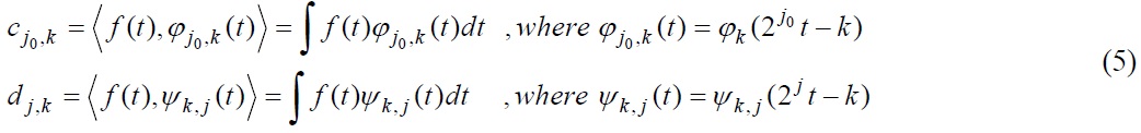
The scaling function φ of Eq. (4) covers the coarsest function space and remaining function space of higher resolution is to be covered by the wavelet function ψ with successive scaling and translating. The coefficient in this wavelet series is called wavelet transform of the function f(t). Since the scaling and wavelet functions are all orthogonal with each other, the coefficients can be calculated through the inner products between the function f(t) and scaling and wavelet functions, as shown in Eq. (5).

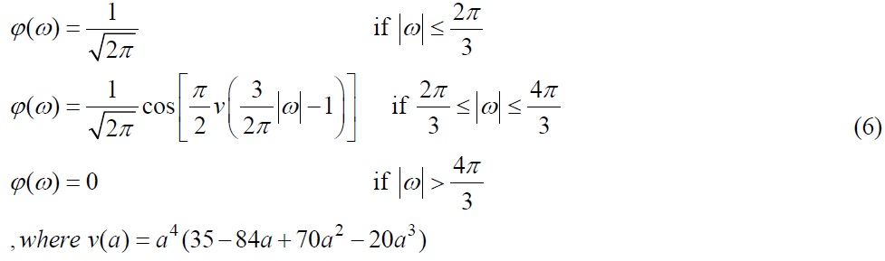
Meyer wavelet is one of the early wavelet functions and the Fourier transform of the corresponding scaling function is defined by Eq. (6).

The wavelet function is then defined by Eq. (7).

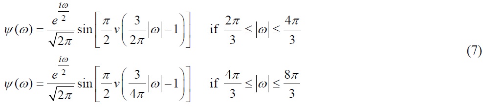
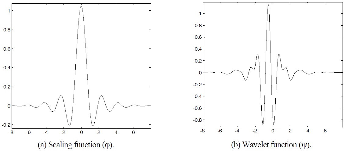
The frequency domain representation of the scaling and wavelet functions clearly tells that the functions are filter banks. The time domain representation of the scaling and wavelet function are shown in Fig. 5 and this functions can be achieved by taking inverse Fourier transform of the Eqs. (6) and (7). The Meyer wavelet function is not compactly supported but it decays faster than any inverse polynomial.

Fig. 6 shows an example of the time and frequency domain representation of Meyer wavelet function up to level 5 when sampling frequency is 2.8 kHz, which means that the shift interval of the wavelet function of the highest frequency band, i.e. level 1, equal to that given sampling frequency. The sampling frequency 2.8 kHz corresponds to the 20 kHz model scale sampling frequency when the model scale is 1/50. Level 5 is the starting scale and level 4 is the one obtained by scaling the level 5 wavelet function by half. Level 3, 2 and 1 are those obtained by successive scaling of the previous wavelet function by half. As the Fourier transform of the wavelet function, given in Eq. (7), tells, each wavelet function forms the filter bank, each of which covers some frequency band depending on the level of the wavelet function. The central frequencies, which are the main frequency component of the highest contribution of each wavelet functions, are 938.14, 469.07, 234.54, 117.27 and 58.63 Hz respectively.

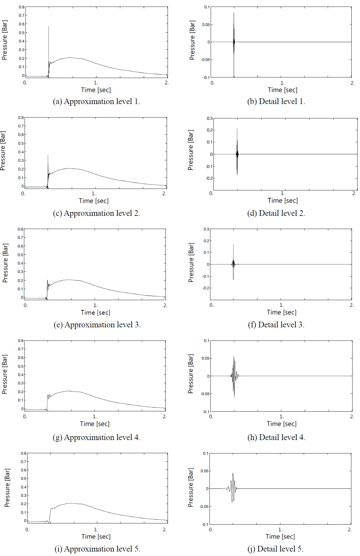
Fig. 7 shows an example of the sloshing impact signal, which is selected out of the long measured signal of 1/50 model scale. A graph shown in the small box at upper right corner shows the magnified view zooming in the impact moment. The details of the experiment from which the signal is chosen, will be discussed in the later stage. Fig. 8 shows the signal decomposition using the wavelet functions of 5 different scale shown in Fig. 6. The approximation level 1, shown in Fig. 8(a) is the signal after the level 1 wavelet function, shown in Fig. 8(b), has been filter out. The detail level 1, shown in Fig. 8(b), is the summation of the wavelet function of level 1 deployed in time. Fig. 8(c) to (j) is the successive filtering process using the next higher level, or lower frequency, wavelet functions. In the long run, the original signal is decomposed into approximation level 5, shown in Fig. 8(i), together with five details of level 1 to 5, shown in Fig. 8(b), (d), (f), (h), (j) respectively.

Therefore, the original impact signal, denoted by p(t), can be expressed as,

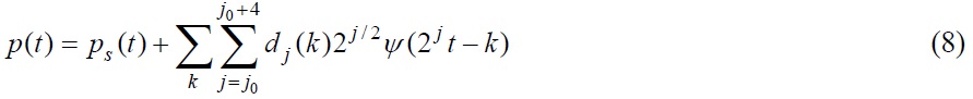
where ψ(2^jt-k) is the 5-(j-j₀) th level wavelet function shifted by k and the function p_s(t) is the one shown in Fig. 8(i).

As was mentioned before, the newly developed strength assessment procedure presented in this paper is motivated by the work of Kim and Kim (2007) who proposed a simplified method to calculate the structural response of the structure under sloshing impact load. A novelty of the present method is the application of wavelet transform for signal decomposition and response synthesization, which is numerically more efficient than the triangular impulse used by Kim and Kim (2007). The merits of the proposed method are mainly on the superior flexibility of the wavelet transform which eventually leads to the minimum number of basis, as well as the structural response calculation using steady state dynamics, rather than transient one.

The dynamic effect of the sloshing impact signal is closely related to the dynamic characteristics of the structure that is supposed to be exposed to the impact load. For example, if the lowest natural frequency of the structure is 1 msec, the sloshing impact load whose rise time is far longer than 1 msec, does not induce any dynamic effect. So, the sloshing impact pressure which varies in a rather slow manner compared to the natural period of the structure can be considered to be static one. Relying on this, it is very efficient to decompose the original sloshing impact signal into slowly varying one and rapidly varying one. The dividing frequency may be determined based on the lowest natural frequency of the structure. By doing this, the slowly varying impact signal and rapidly varying impact signal can be handled separately, that is to say, the slowly varying one as the static load and the rapidly varying one as the dynamic load. Fig. 9 shows the signal decomposition into slowly varying one and rapidly varying one based on the frequency band of the Meyer wavelet function of different scale. The slowly varying signal shown in Fig. 9(c) is the same one as shown in Fig. 8(i) and the rapidly varying signal shown in Fig. 9(b) is the summation of the all the details shown in Fig. 8. As the central frequency of level 5 wavelet function corresponds to 58.63 Hz, i.e. 17 msec in term of the period, the slowly varying signal includes the sinusoids whose periods are mainly longer than 17 msec. Considering the stiffness and mass characteristics of the insulation box of GTT NO96 cargo containment system, it is reasonable assumption that level 5 for this particular case is right choice as the cut-off between static and dynamic. Usually, the response of the insulation box becomes almost static once the rise time of the sloshing impact load is larger than 6 msec (Kim et al., 2010).

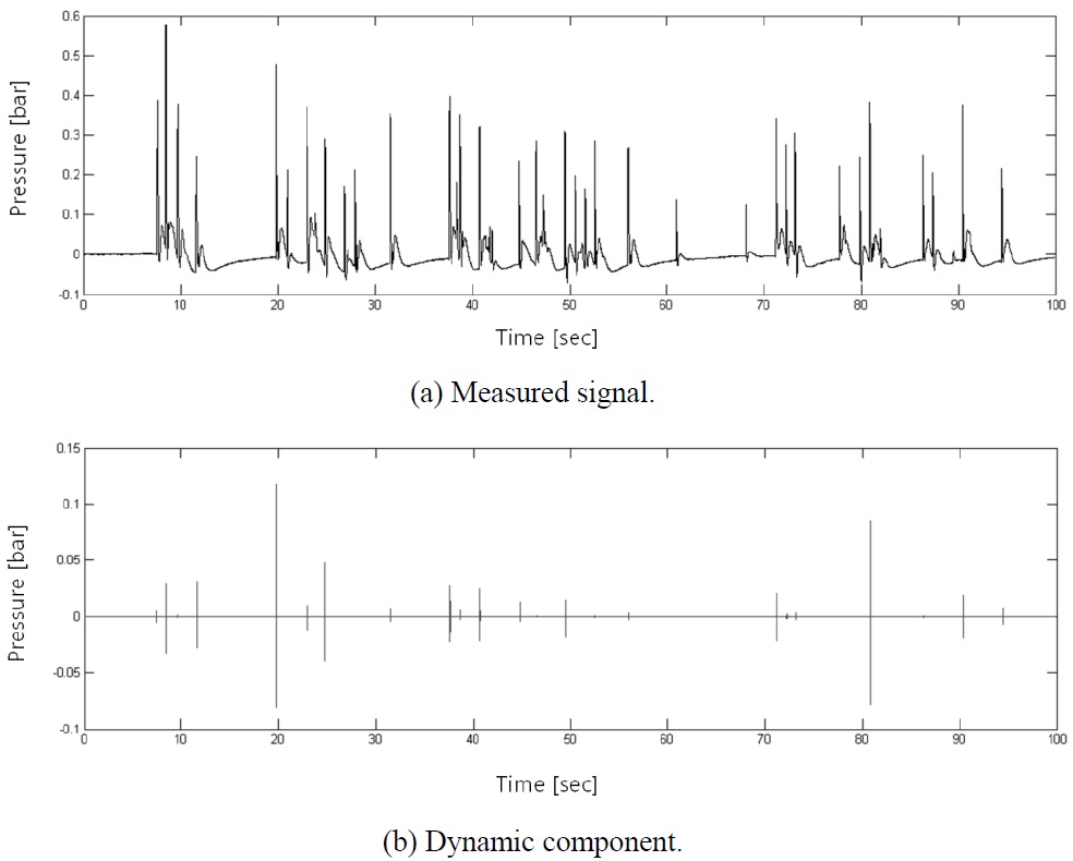
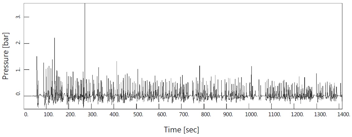
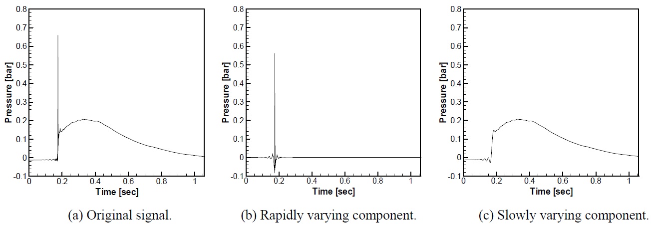
The main focus is on the rapidly varying signal which is going to be handled as the dynamic load acting on the structure, whereas the slowly varying signal is handled as the static load which is easy to treat. It can be said that, by separating the load into static and dynamic one, the overall efficiency of the signal decomposition and the response calculation becomes really high. This is due to the fact that the dynamic load is retained within very short time duration, which means the data that have to be handled with special attention is minimized. Fig. 10 shows relatively long time history of sloshing impact signal measured on 1/50 scaled model. The measured signal shows 34 significant impacts but after filtering out the static signal, the significant impact number becomes only 16. This means that the other 18 impacts are static loads whose rise time is larger than 17 msec. Looking at the original signal shown in Fig. 10(a), the impact number 2 is the highest but when it comes to the dynamic component, impact number 5 is the highest. In terms of the structural response, no one can clearly dictate that the impact number 2 is more critical than the impact number 5 since the dynamic impact always entails dynamic amplification effect, as may be the case of impact number 5.

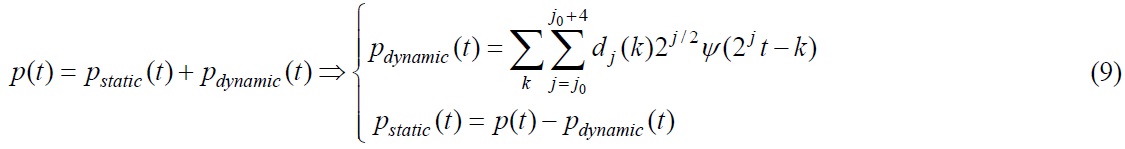
The dynamic component, or rapidly varying signal, is further decomposed into wavelet basis function as described in Fig. 8. This is achieved through the wavelet transformation process, hence the wavelet coefficients d_j,k of each wavelet function of different scale are stored together with its location information, k. The entire decomposition process can be explained by the Eq. (9).

The wavelet response function is defined as the response of the system under each wavelet function of different scale. Provided that the wavelet response function is given, the response of the system under sloshing impact pressure of arbitrary time history can be obtained by synthesizing the wavelet response function. In order to build the wavelet response function, the structural analysis needs to be carried out under each wavelet function of different scale. This can be achieved by analyzing the system using structural finite element analysis either in time and frequency domain. Since the Meyer wavelet is well represented by the pure trigonometric functions as described in Fig. 6(b), the wavelet response function can be obtained in frequency domain considering the numerical efficiency that frequency domain approach has.

The FE model of NO96 insulation box is same as the one shown in Fig. 3(b), maintaining the other details same. The sloshing impact pressure is assumed to act on the top surface of the box. Both explicit transient dynamic FE analysis and frequency domain steady state dynamic analysis have been carried out and the correspondence between the two different results is cross compared. The time history of the sloshing impact pressure for the transient dynamic analysis and the frequency contents of the sloshing impact pressure for the steady state dynamic analysis for each wavelet function of different scale are those given in Fig. 6. The vertical component stress at the location A, shown in Fig. 3, is selected and used for the result comparison. The analyses have been carried out using the commercial FE program ABAQUS Ver. 6.8.

As was mentioned before, the Meyer wavelet is not compactly supported, so the truncation has been made for the time domain transient dynamic analysis considering the fact that the decay rate of the Meyer wavelet is rather fast. The justification for this truncation can be automatically made since the dynamic pressure, shown in Fig. 10(b), clearly demonstrates that the sloshing impact event can be handled independently without interaction among them. This is possible due to the fact that the impact event takes place with some time interval, which is long enough from the viewpoint of the dynamic oscillation of the structure. For the frequency domain calculation, frequency component of wavelet basis function along with the phase angle was input to the FE program in the form of real and imaginary number, and the output given in frequency domain was transformed into time series by combining the modulus and phase angle. For the time domain calculation, the direct discretized time series of the wavelet basis function was applied to the FE model and the response time series is obtained accordingly. The structural damping is assumed to be about 5% of its critical damping of the lowest vibration mode for both time and frequency domain approaches.

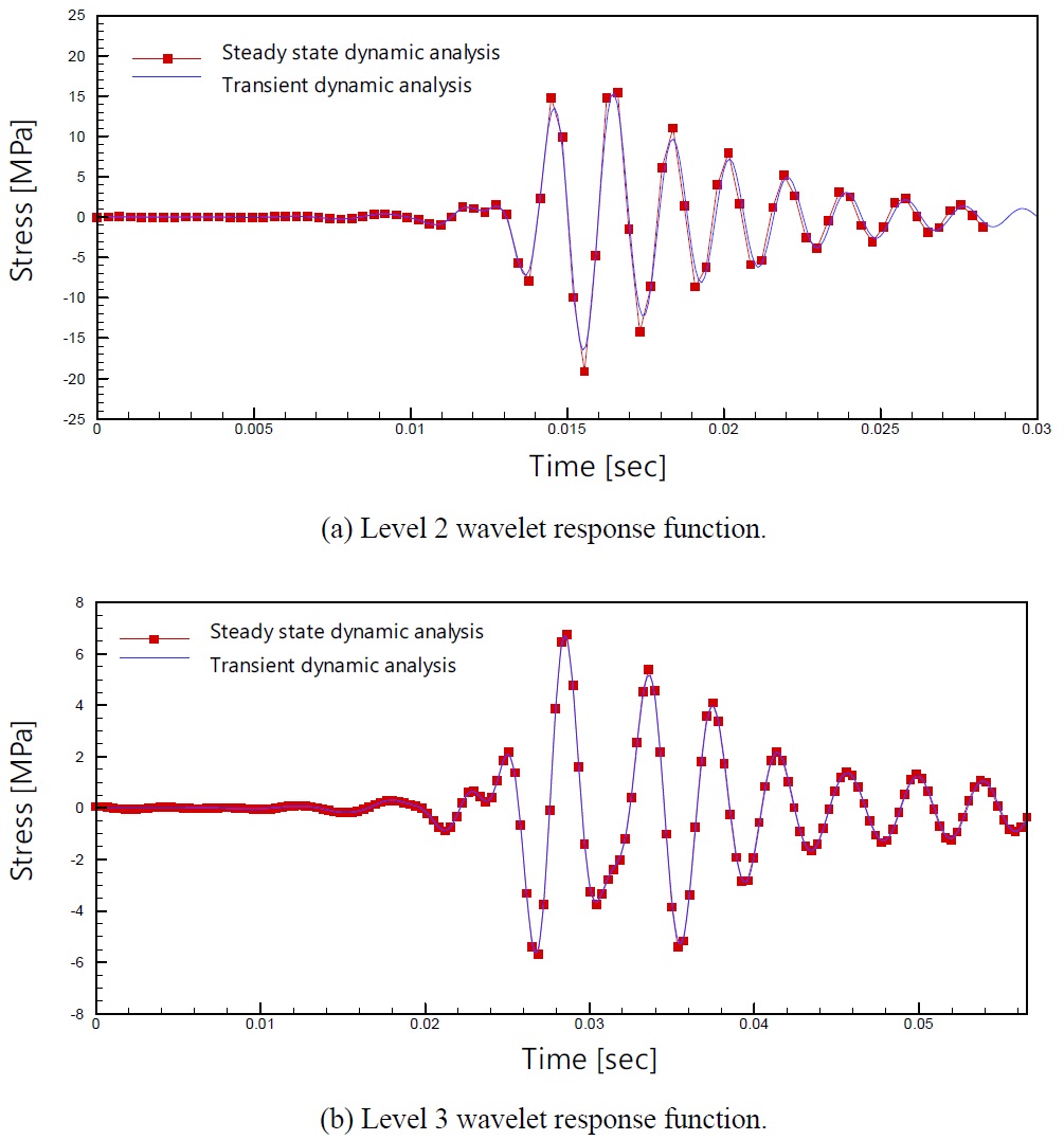
Fig. 11 shows the wavelet response function of level 2 and level 3. The curve with dots is the result obtained by running steady state dynamic analysis and the plaine curve is the result obtained by transient dynamic analysis. It can be seen that two results obtained from two different numerical approaches give almost identical results. From practical point of view, the wavelet excitation of level 2 and 3 are the main contributor to the spiky impact signal when sampling frequency is 20 kHz, so these two are of the prime importance out of all 5 levels.

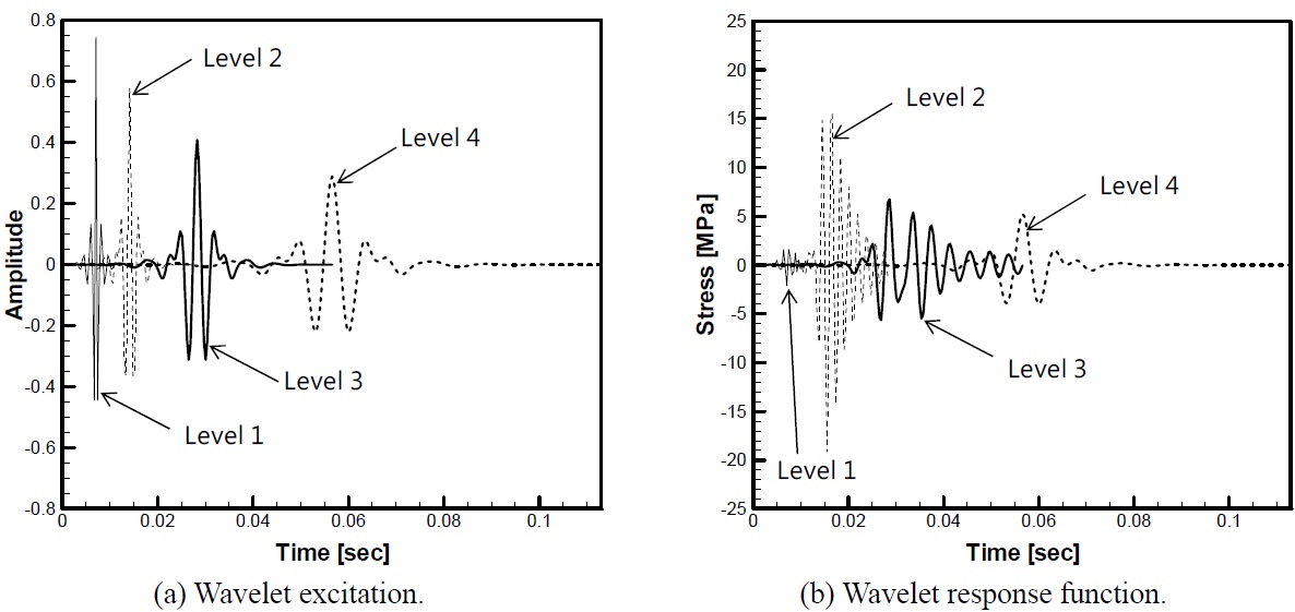
Fig. 12 summarizes the calculated wavelet response function compared with the wavelet excitation from level 1 to 4. It can be clearly seen that the dynamic effect is very pronounced for the level 2 and 3. The response under level 4 is already static-like so that the shape of stress signal is not so much different from the excitation, and this indirectly tells that the stress response under level 5 is static enough. For the level 1, the structural response is rather calm compared to the level 2 case considering the larger excitation magnitude of level 1 shown in Fig. 12(a). This is due to the fact that the frequency of level 1 excitation is too high to influence the structure, that is to say, the impact pressure disappear so quickly that there is not enough time for the structure to feel the excitation. It may be said that the small magnitude of the wavelet response function under level 1 excitation enables us to filter out level 1 frequency band out of the original signal without losing the accuracy of structural response. Even if the intensity of level 1 component is rather high in some cases, filtering out the level 1 component usually does not distort the structural response that much in case that the underlying structure is the GTT NO96 insulation box.

The response synthesization of the dynamic process is similar to the convolution integral of impulse response function, and is given as Eq. (10) under j-th level wavelet excitation. The stress time history, at a given location under wavelet function excitation of j-th level, can be obtained by convolution type summation of the wavelet response function and wavelet coefficient.

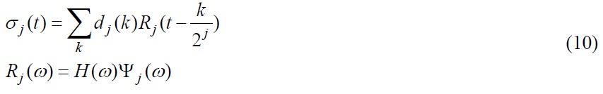
Here, ψ_j(ω) is the Fourier transform of the wavelet function of j-th level, H(ω) is the linear transfer function of the system and R_j(ω) is the Fourier transform of the wavelet response function under the wavelet function excitation of j-th level. The whole response of the system under sloshing impact pressure of arbitrary time history can be obtained by integrating the stress time history of j-th level together with the static response.

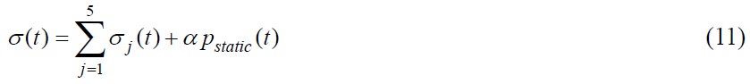
The constant α in Eq. (11) is the transfer function of the system under static load, so factoring the static pressure with α directly gives the stress at corresponding location.

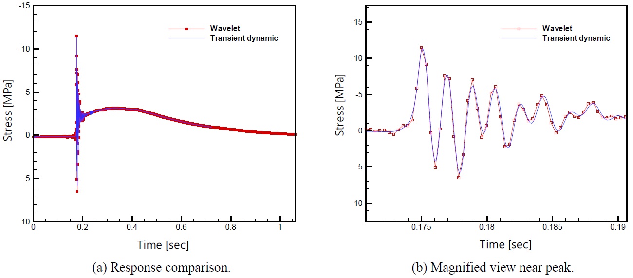
To check the validity of the proposed scheme, the response of the GTT NO96 insulation box shown in Fig. 3(b) is again analyzed under a single impact event shown in Fig. 7. Fig. 13 shows the response comparison between the two methods. The curve with dots is the analysis result obtained through the response synthesization method described above, and the curve without mark is the analysis result obtained through the explicit transient dynamic analysis. Fig. 13(a) demonstrates that the overall tendency between the two results matches very well, and Fig. 13(b) confirms that the detail responses of the two results near the response peak taking place around 0.18 sec also correspond well.

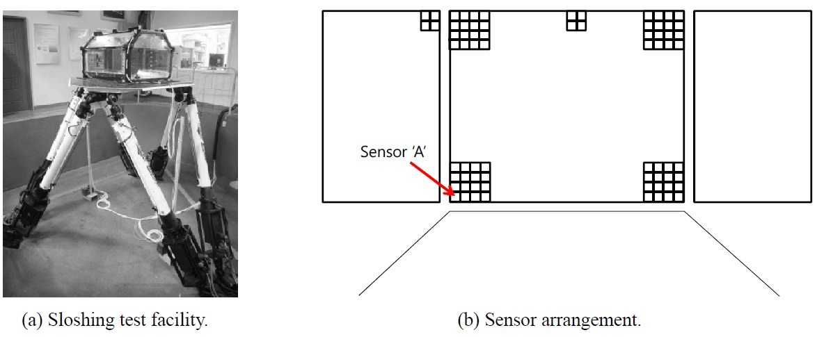
For the cross comparison of the current method with traditionally used load based approach, a set of pressure time history is selected from the sloshing model test of 1/50. The model test is about the 138 K LNG carrier, which is moving forward with the speed of 5 kts and exposed to the bow quartering sea with 95% of filling level. The sea state the vessel is subject to is H_s = 9.5 m and T_z = 7.5 sec. The test was run for 5 hrs. full scale time. The pressure sensors were installed at three corner of the upper ceiling in the form of 4 by 4 cluster, together with some other areas as shown in Fig. 14. Since the spatial distribution of the pressure is not important factor in the validation of the current methodology, it is assumed that the pressure time history picked at

one of the sensors acts on the entire top surface of the GTT NO96 insulation box. Pressure sensors of ICP type by Kistler Instrument Corporation were installed on the model tank. The diameter of the sensor is 5.54 mm which corresponds to the 0.227 m in full scale matching the area less than 1/4 of a single standard NO96 insulation box in full scale. The natural frequency of the sensor is 300 kHz so that the interaction with impact is not expected. The sampling frequency is 20 kHz. Fig. 15 shows the pressure time history that is picked up at the sensor location ‘A’ denoted by an arrow in Fig. 14.

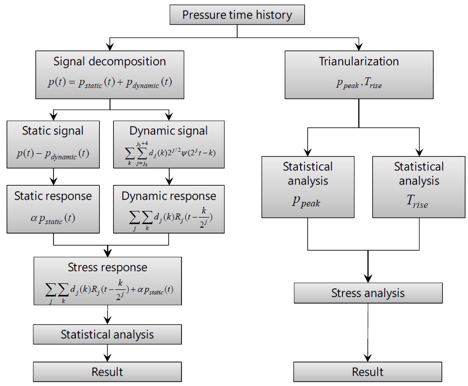
The analysis results from the developed approach were compared with those from the traditionally used load based approach, where an arbitrary impact event is parameterized by the peak value and pressure rise time assuming that the signal is traingular. Fig. 16 shows the procedure of two methods for calculating the response of the structure under a sloshing load, the proposed wavelet based method on the left side and the traditional load based method on the right side. Both methods start with the same pressure load history shown in Fig. 15.

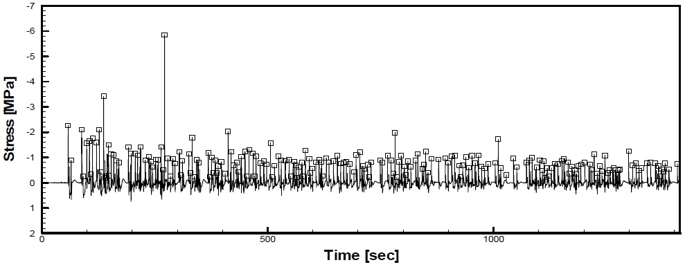
As was explained before, the developed approach splits the pressure signal into slowly and rapidly varying component respectively in order to take advantage of the static nature of the slowly varying component. For the slowly varying component, the stress response can be easily obtained by the simple static analysis since no dynamic effect is present in the response of the structure. For the rapidly varying component, the wavelet transformation method is used to decompose the signal into its wavelet basis functions and the wavelet response functions are sought and used for the response synthesization considering the dynamic effect of the underlying structure. Then the total response can be calculated by summing up the static and dynamic response. Then the stress time history was statistically analyzed to extract the extreme value. Fig. 17 shows the stress time history which is converted from the pressure time history shown in Fig. 15, following the procedure shown in Fig. 16. Dots are the stress peaks that is used for the statistical analysis in the following step.

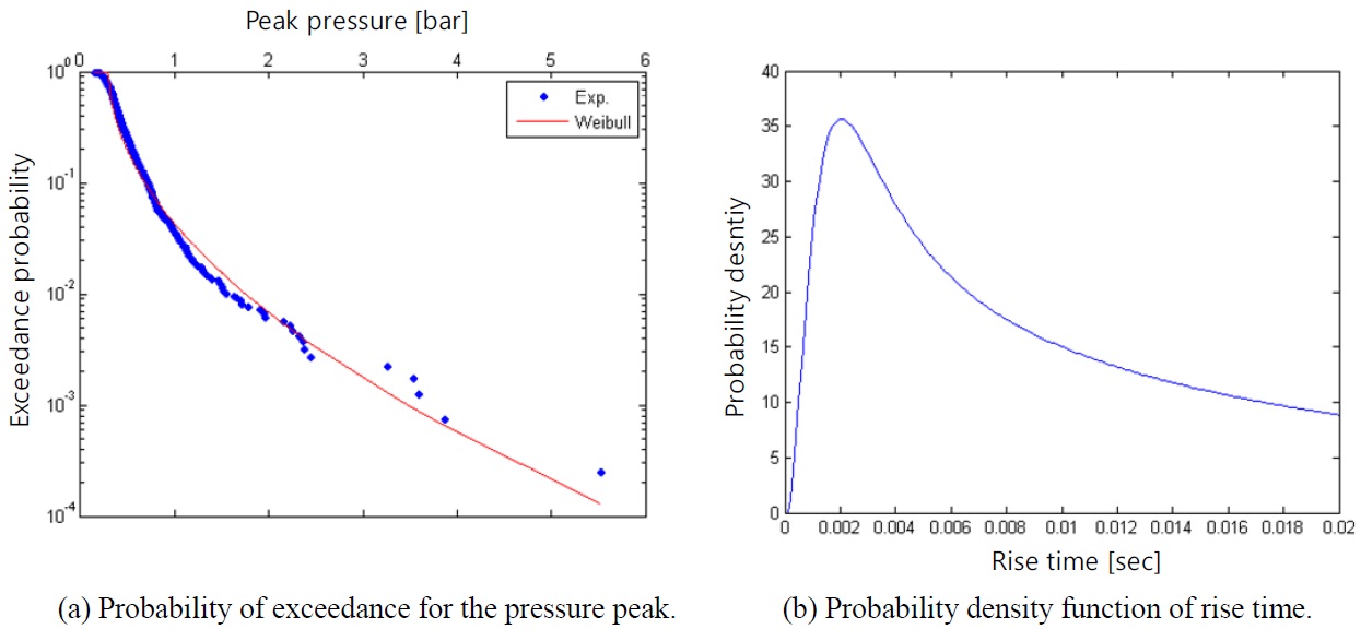
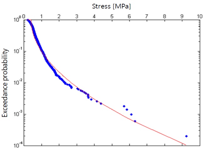
One of the key parts of the analysis is the statistical analysis through which the most probable maximum stress value within a given time duration is derived. The histogram of the identified peaks is derived then the probability density function is determined by curve fitting. Normally, for extracting the extreme value, 3 parameter Weibull distribution is used as shown in Eq. (12).

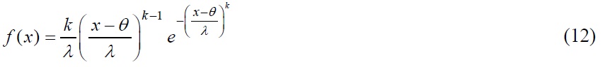
where k is the shape parameter, λ is the scale parameter and θ is location parameter respectively (DNV, 2006). The statistically meaningful 3 hrs. extreme value can be derived based on the exceedance probability function along with the exceedance probability value that corresponds to 3 hrs. Fig. 18 shows the plot of the probability of exceedance for the stress peaks found in the stress time history shown in Fig. 17, together with its 3 parameter Weibull fit. The 3 hrs. maximum stress value is obtained by the fitting turned out to be 6.84 MPa in compression.

In case of load based approach, the most probable 3 hrs pressure peak value was extracted through the statistical analysis. Representative rise time was determined based on the separate statistical analysis on the rise time itself. The representative rise time was selected at the location where probability density of the rise time itself peaks. It was accepted to be reasonable to use the rise time data set whose corresponding pressure peak values are within the top 10%. Fig. 19 shows the probability density function of the rise time of top 10%, together with the probability of exceedance for the pressure peaks. The modal rise time turned out to be about 2 msec and the 3 hrs. maximum pressure peak is around 4 bar.

The derived rise time and the peak pressure forms a single representative triangular impulse load, and this is applied on the top surface of the GTT NO96 insulation box model. The explicit transient dynamic analysis has been carried out and the maximum stress out of the transient stress response at given location is picked up. This value turned out to be 5.85 MPa in compression. The value obtained by the load based approach predicts the stress level about 17% lower than the one obtained by the proposed wavelet based approach. It is somewhat surprising that the prediction given by the load based approach is not conservative one, and this suggests that the current load based approach needs some modification in its procedure to guarantee the conservatism and the proposed response based approach may play some important role for that.

There are some modeling uncertainties related to the temporal characteristics of the sloshing impact pressure in the current design procedure of the strength assessment of the LNG cargo containment system. To avoid the issues, a new response based strength assessment procedure was developed by using the wavelet transform technique. Based on the studies carried out in this paper, following conclusions are derived.

Current load based approach idealizes the sloshing impact pressure with simple triangular shapes, and this introduces some modeling uncertainties related to the temporal characteristics. Those are the ambiguity of the rise time definition, the effect of decay time and the possible load interaction effect and so on. The response directly obtained from the transient FE analysis also confirms that the above mentioned uncertainties produces significant differences of the structural response of the underlying structure that is exposed to the impact pressure.

The rapid response calculation procedure has been developed in this paper using the wavelet transform technique. First of all, the long duration sloshing impact signal is decomposed into the slowly varying and rapidly varying component with its cutoff frequency determined by the natural frequency of the underlying structure. This guarantees that the structural response under slowly varying component may be regarded as static one, whereas the dynamic response is induced only by the rapidly varying component. The dynamic response under rapidly varying component is obtained by convoluting the wavelet response function of the system and the wavelet transform coefficient, and the whole response is synthesized by superimposing the static and dynamic response.

The response calculated by the developed approach was directly compared with the results obtained from direct transient dynamic FE analysis. It was confirmed that the developed approach produced almost identical results with those obtained by direct FE calculation, as was expected.

A case study has been carried out for the pressure time history measured from the model test of 138 K LNG carrier, and comparison was made between the proposed method and conventional load based approach. It turned out that the 3 hrs maximum stress obtained by the proposed method was larger than the one obtained by the load based approach by 17%. It may be concluded that the load based approach which relies on the separate statistical analysis for both rise time and pressure peak does not guarantee conservative result.

On top of the benefits that are achievable in the response calculation, wavelet decomposition gives rise to further advantages such as, high data compressibility, enhanced readability of the signal and so on. Also, the wavelet transform result highlights some characteristics of the sloshing impact signal and valuable information can be derived out of it, such as the identification of the dynamic components, which is hard to recognize in the time history of the signal.