Due to the tremendous increase of energy consumption and worldwide political instability, oil prices have been on the rise. As an effort to overcome the unprecedented high oil prices, many countries have concentrated their efforts in finding energy sources in the Arctic region. To access the abundant natural resources in that region, passage across the Arctic must be established.
Recent global warming has accelerated the melting phenomenon of the Arctic ice and as a result this situation has allowed the human access to the Arctic area. The Northern Sea Route (NSR) along Russia and the Northwest Passage (NP) located near Canada were finally open, allowing fast navigation between the Pacific and the Atlantic oceans. The importance of those two routes can be explained by the enormous amount of natural resources buried in the northern region of Russia and Canada.
Geometrically, the NSR or NP routes are the shorter paths, compared to the conventional route passing through Suez Canal route (Ostreng et al., 1999), which noticeably saves time and expenses. Nonetheless, navigating the NSR or NP is hard to carry out, not only because of the harsh environment but also the restrictions implicitly imposed for political reasons. In particular, the harsh environment results in many technical difficulties that would make it hard for a year-round commercial shipping route.
Simulating possible navigational routes is difficult and challenging but extremely beneficial to the shipping companies. Therefore, before dispatching the icebreakers or ice-strengthened vessels to the Arctic region, they want to simulate the technical and economical feasibilities based on precise ice and environmental data.
One of the crucial requirements required to overcome the technical challenges along the Arctic route is the accurately predicting the environmental conditions in the region. Traditionally, obtaining the environmental data such as ice concentration, thickness, strength, visibility, and so forth has not been an easy task. The traditional method of observation is not only obsolete but also unreliable. Recent development of technical equipment utilizing electromagnetic device, satellite, or sonar has upgraded accuracy and effectiveness in measuring the environmental condition. These high tech methods, however, still have many problems with respect to reliability.
To compute the navigational route, it is necessary to have a so-called transit model, which describes every piece of information required for navigation. La Prairie et al. (1995) suggested a transit model to estimate the cost by considering the relationship between the thrust of a ship and ice resistance. Their model is very complicated to use. Another big leap started with the launch of the International Northern Sea Route Programme (INSROP). It is a numerically analyzed model that determines the optimal route by estimating the distance, speed, and icebreaker fee (Patey and Riska, 1999; Kamesaki et al., 1999). Unfortunately this collaborating work was discontinued in 1999. On the other hand, CRREL (U.S. Army Cold Regions Research and Engineering Laboratory) developed a NSR transit model (Mulherin et al., 1996). They described the ice model using probabilistic distribution and utilized Monte Carlo iteration to find routes. A modified CRREL model was suggested by the authors (Choi et al., 2010; Ha et al., 2011). This model basically adopted the concept suggested by CRREL, but included more practical data omitted in the CRREL model. It used a direct method to compute the route instead of the lengthy Monte Carlo approach.
A critical disadvantage encountered in the previous efforts is that the user must provide accurate data of sea ice along the routes in NSR and NP. The data must be updated on a regular basis prior to voyages. Real-time update of ice and environmental data transferred from a satellite, for example, may be the most desirable scenario but can be risky and unreliable.
An approach to overcome the above disadvantage is to prepare a more versatile model that accurately and dependably describes the sea ice condition. Possible candidates of those models would include an analytical model obtained by solving a governing equation or a numerical model by simulating the current data. Although it would be premature to assert that these models fully describe the ice condition with accuracy, they provide an introductory step in accommodating a comprehensive transit model.
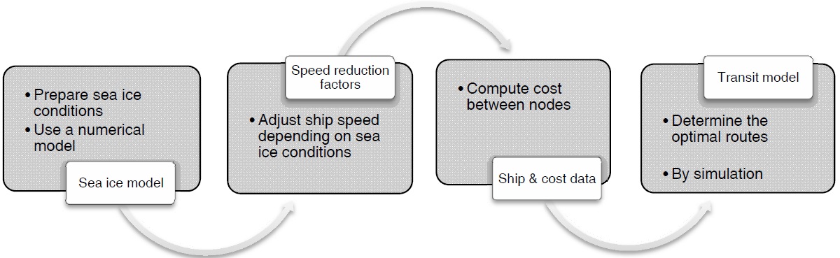
Another goal of the work is to establish a simulation system that computes the optimal routes in the Arctic region. Obtaining an optimal route requires a systematic approach in setting up a computerized system that encompasses various different techniques such as database, graphical user interface, graph theory, and the concept of simple user interaction. A simulation system built upon the basic technical tools is developed. The organization and internal process of the simulation system are illustrated in Fig. 1.
In this paper, a simulation system based on a sea ice model that solves a general circulation method is presented. Each major concept shown in the Fig. 1 will be dealt with. Establishment of a numerical sea ice model that will be used in the transit simulation is explained in the upcoming section. Construction of a huge database for ice and environmental data is addressed and followed by the discussion of a method that finds an optimal route. The simulation of the transit model is executed and its results are analyzed.
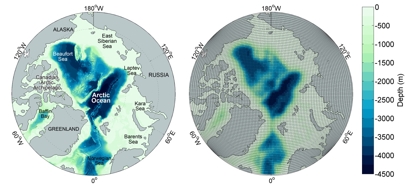
The distribution and variation of the sea ice in the Arctic Sea with an ice-coupled ocean general circulation model (OGCM) have been simulated. The OGCM used in this work is the regional ocean model system (ROMS) version 3.4, which is a three dimensional, s-coordinate, primitive equation for an ocean model widely used by the scientific community for various applications. The sea ice module of the ROMS includes sea ice dynamics and thermodynamics. The sea ice dynamics are based on an elastic-viscous-plastic rheology of Hunke and Dukowicz (1997) and Hunke (2001) including ice momentum equations as well. For ice thermodynamics, two ice layers and a single snow layer are used to solve the heat conduction equation (Mellor and Kantha, 1989). The snow layer possesses no heat content but plays a role as an insulating layer. Surface melt ponds are included in the ice thermodynamics. Further details can be found on the ROMS web site (http://www.myroms.org).
The numerical model or numerically simulated model (referred to the model throughout this section) covers the Arctic Sea north of 65°N with an orthogonal curvilinear grid system. The horizontal grid size ranges from 41 to 63
The model uses Flather (1976) and Chapman (1985) boundary conditions for barotropic normal velocity components and the sea surface elevation along open boundaries. Temperature, salinity, and baroclinic velocity components at open boundaries are calculated with a radiation condition suggested by Marchesiello et al. (2001). The 6-year (2004-2009) monthly mean HYbrid Coordinate Ocean Model / Navy Coupled Ocean Data Assimilation (HYCOM/NCODA) Global 1/12° analysis data are used to specify input values of temperature, salinity, sea surface elevation, and velocity components for boundary conditions.
SIMULATION RESULTS OF COUPLED ICE-OCEAN MODEL
To initialize the model, the model is spun up for 30 years with daily mean atmospheric fields from the European center of medium range weather forecasting Re-Analysis Interim (ERA-Interim) averaged over the period of 1990-2009. During the spin-up mode, temperature and salinity are set to values from the monthly climatology data provided by the Polar Science Center Hydrographic Climatology (PHC) (Steele et al., 2001) with a relaxation scale of 30 days. After spinning up model, a hindcast simulation is conducted from January 1, 1990 to the end of 2009 with a 12-hourly atmospheric forcing and no climate restoring for temperature and salinity.
>
Sea ice concentration and extent
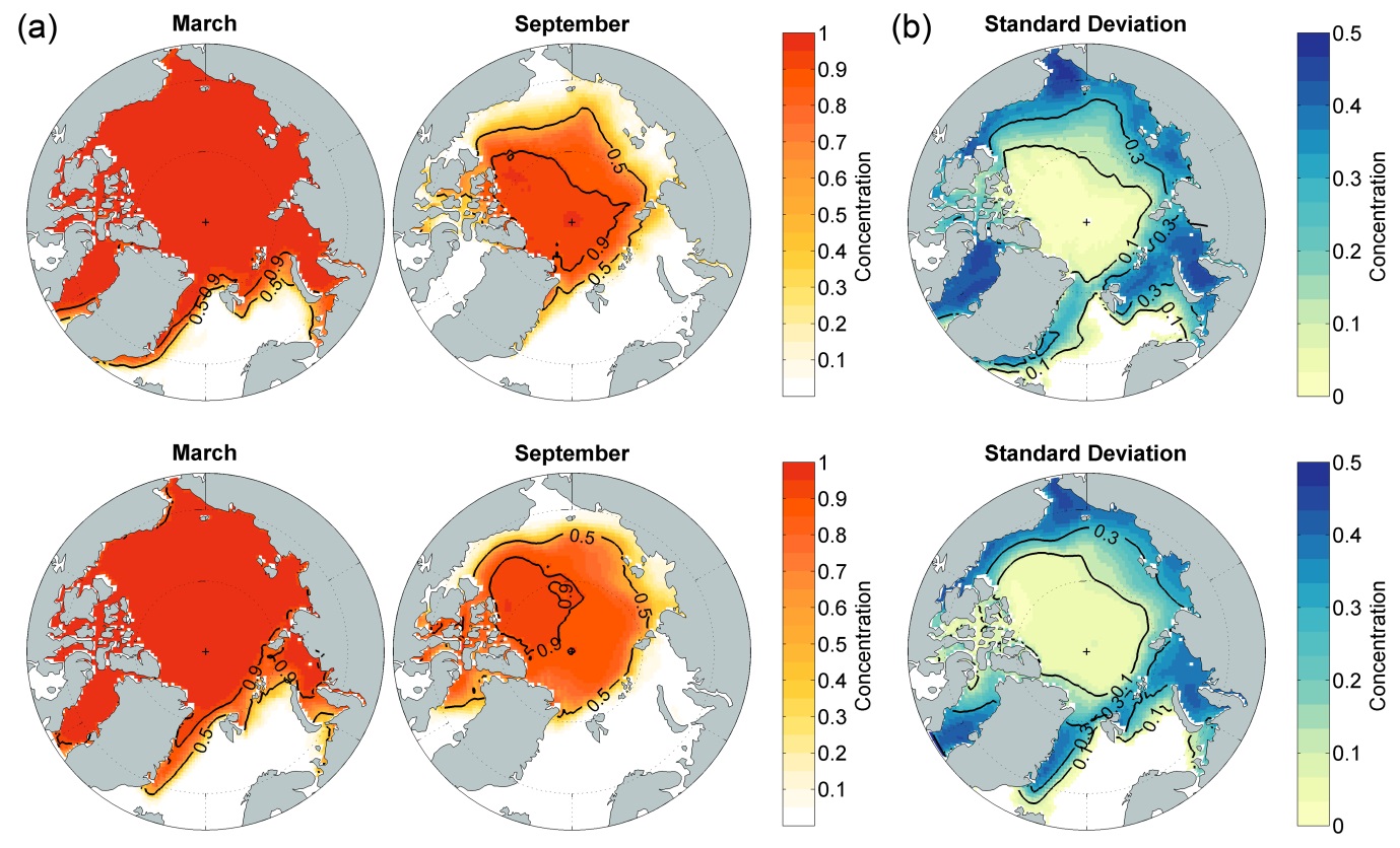
Fig. 3(a) shows the two sets of sea ice concentrations in March and September. The upper set are observed ice concentrations obtained from the Met Office Hadley Center’s sea ice and sea surface temperature data set (HadISST) (Rayner et al., 2003) over the period 1990-2008, while the lower set are obtained from our numerical model. In March, the simulated fields show a good agreement with observed one except that the model somewhat underestimates sea ice concentration in the Kara Sea south of Severnaya Zemlya islands. Both results show sea ice concentrations near unity over most of ice-covered area. Differences between two sets become noticeable in September. The model appears to underestimate the sea ice concentration while its extent is larger than the observed one. The sea ice edge is extended further southward in the East Siberian Sea and Laptev Sea. The model also shows less summer melting in Baffin Bay and Canadian Arctic Archipelago. It may be partly due to the coarse grids that are not sufficient enough to correctly resolve geography.
Fig. 3(b) shows the standard deviation of monthly sea ice concentrations over the 19-year averaged fields during the same period. The standard deviation in this case mainly indicates the range of seasonal variability, though the inter-annual variability can be included to some extent. The model seems to reproduce the seasonal variability well along the sea ice edge in September except relatively lower variability in the Kara Sea and Baffin Bay.
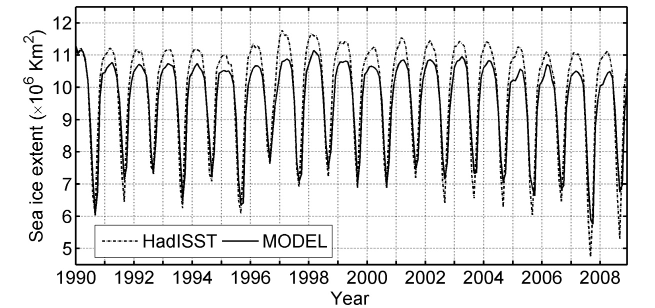
Fig. 4 shows the comparison of modeled and observed sea ice extent. The sea ice extent is defined as an area whose ice concentration is greater than 0.15. The simulated result seems to track the seasonal and inter-annual variations of sea ice extent although their amplitudes are smaller than the observed one. The 19-year averaged sea ice extents for observation are 11.26 × 10⁶
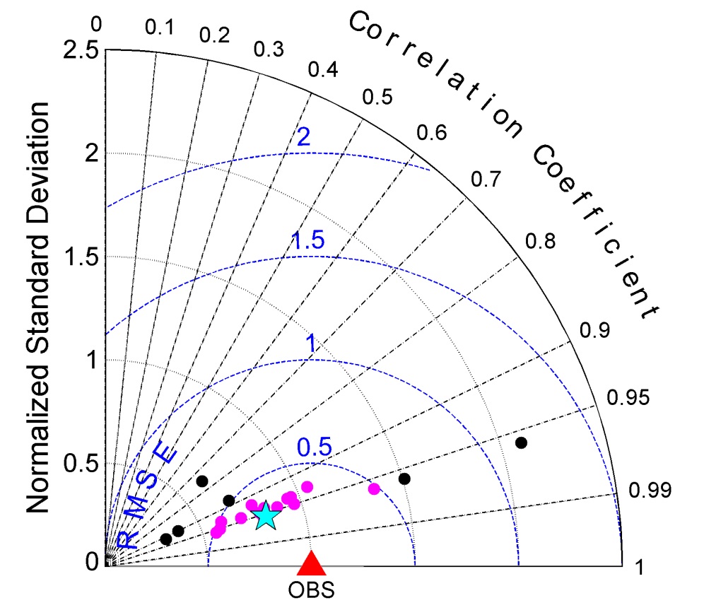
To evaluate the model performance, the simulated results are compared to those in the Intergovernmental Panel on Climate Change Assessment Report 4th (IPCC AR4), which includes all twenty models simulating the Arctic sea ice with a range of grid resolutions from 0.2° to 5° (Fig. 5). The star marker denotes our model result and the triangle the observed value. The darker dots indicate the results of all twenty models in the IPCC AR4 while the lighter dots note models that have RMSE less than 0.5.
For a quantitative comparison, a Taylor diagram using the time series of monthly sea ice extent is used. The Taylor diagram is a useful tool to show the relative merits of models simultaneously comparing normalized standard deviation (NSD), rootmean- square error (RMSE), and correlation with observation (Taylor, 2001).
In Fig. 5, RMSE and NSD are normalized by the observed standard deviation (1.72 × 10⁶
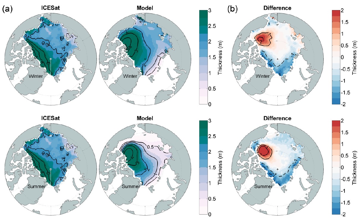
Fig. 6(a) shows the simulated sea ice thickness and satellite data, obtained from the Ice, Cloud, and land Elevation Satellite (ICESat). Since the ICESat data set consists of five winter (February?March) and summer (October?November) campaigns during the period of 2003-2008, the modeled sea ice thickness is averaged. The differences between the two sets are calculated by subtracting the observed fields from the model results (Fig. 6(b)).
Both ICESat data and model show that relatively thicker ice (≥ 2
CONSTRUCTION OF SEA ICE DATABASE
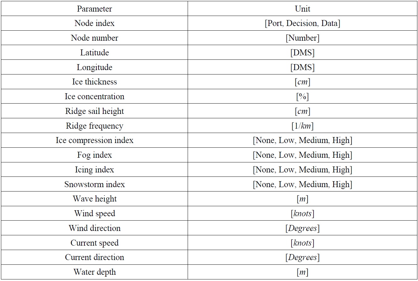
After the sea ice model has been numerically simulated, results need to be stored for later retrieval. A database containing all the data of sea ice information is constructed for the purpose of efficient manipulation of heavy data. Those data include thickness, concentration, temperature, current, and salinity of the Arctic sea ice at 5,352 nodes of an orthogonal curvilinear grid system above 65°N, between year 1990 and 2009. At each node, other data such as latitude, longitude, and environmental values are also available. All ice and environmental data stored at a node are tabulated in Table 1.
The node index indicates that a node can be categorized as port, decision, or data. The decision node implies that the ship does not stay but passes through the node. The data node is artificially inserted and used only for internal interpolation. The size of obtained data is so huge that they should be effectively stored for later update and retrieval. In the simulated model, the numbers of nodes for port, decision, and data are 21, 50, and 5281, respectively.
A handy way to store the huge series of data is to use an open source such as MySQL (http://www.mysql.com). It is a fast growing database, known as an economic and efficient tool in establishing a scalable database construction and its applications. Moreover, its community edition is freely downloadable. On the other hand, Microsoft ActiveX Data Objects (ADO), a set of COM (Component Object Model) based objects, has been shown to be effective with respect to its performance and integration with the graphical user interface in Windows computing environment. Either MySQL or ADO shows decent performance.
[Table 1] List of data stored at a node.

List of data stored at a node.
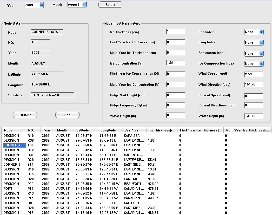
Fig. 7 shows a dialogue pane that lists the sea ice data satisfying the conditions given by the user. The purpose of the user interaction is to offer a chance to view and modify the specific data upon the user’s interest. The user is allowed to choose one or multiple years. If multiple years are selected, their average is used in the computation. It has been found to be useful when the user wants to simulate an artificial sea ice condition by modifying some parts of data.
DETERMINATION OF OPTIMAL ROUTES
The optimal route used in this work is the route that costs the least. The faster the voyage, the more cost efficient the expenses. Thus the optimal route is determined by the ship speed. If the ship speed increases, it takes fewer days and thus the overall cost decreases.
To derive the operating cost, various factors are considered. Main contribution to the cost includes fuel, oil, icebreaker fee, capital and port cost. The fuel cost is the product of fuel consumption rate and fuel price. The operating cost is the sum of crew salary, provisions, maintenance, insurance, and ice pilot fee. The sum of stays at origin, stopover, and destination ports affects to the port cost.
The cost is represented in terms of cruising speed that is calculated by considering all the factors at each node. The cost associated with the cruise speed involves various factors required for the cruise and maintenance of the ship. In this work, the overall cost function introduced by the authors (Choi et al., 2010) is reused, as shown in Eq. (1).

where CF is fuel and oil cost, CO operational cost, CP port charge, CIB icebreaker fee, and CC capital cost. The use of an icebreaker ironically has shown to become the dominant factor in most cases. Therefore, taking a route that avoids the region where an icebreaker must be accompanied is strongly recommended. It should be noted that the use of an icebreaker is a subtle issue that is subject to political negotiation, which is beyond the technical issues addressed here.
The ship speed, which affects the overall cost, uses the concept of base speed. The base speed is determined by the design speed of a ship, ice concentration, and ice thickness. If a ship traverses an ice-free region, the base speed naturally becomes the ship speed. The existence of concentrated ice region or thick and deformed ice causes the speed reduction by applying penalty to the base speed. Other speed reductions considered in this work are due to ice concentration, ice thickness, ice compression, ridge, fog, and other environmental data.
Ice is a dominant contributor to speed reduction. Concentrated and/or thick ice makes the ship slow down depending on its scale. The worst-case scenario is to rent a powerful icebreaker that dramatically increases the overall cost. Table 2 summarizes the adjusted speed due to the thickness and concentration of ice. The basic idea of this speed reduction was borrowed from CRREL but major enhancement was made for more accurate prediction (Choi et al., 2010). The ship should be navigated at its design speed in the ice-free region or when the ice thickness is less than 30
[Table 2] Adjusted speed for thickness and concentration of ice [in knots].
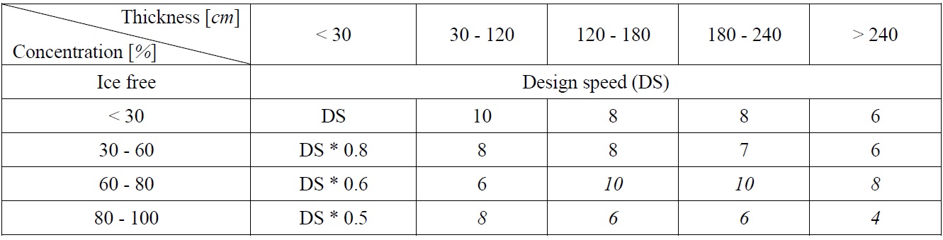
Adjusted speed for thickness and concentration of ice [in knots].
The next speed reduction is due to ice ridges. Ridges form when level ice floes are level ice areas are compressed and sheared by environmental driving forces (Timco et al., 2000). Ridge-building processes are in general complex and involve some rafting in combination with various bending, buckling or crushing failures. The resulting ridge feature contains a large number of ice pieces of varying sizes that are piled in a haphazard manner. Therefore, the existence of ridges becomes a serious obstacle for navigation. The frequency of ridges per unit kilometer and their sail height tabulated in Table 3 determines the possible navigating speed. It should be noted that the existence of large ridges could hinder the voyage itself, causing the ship to make a detour. This roundabout passage is common in winter season.
[Table 3] Speed reduction factors for ice ridges.
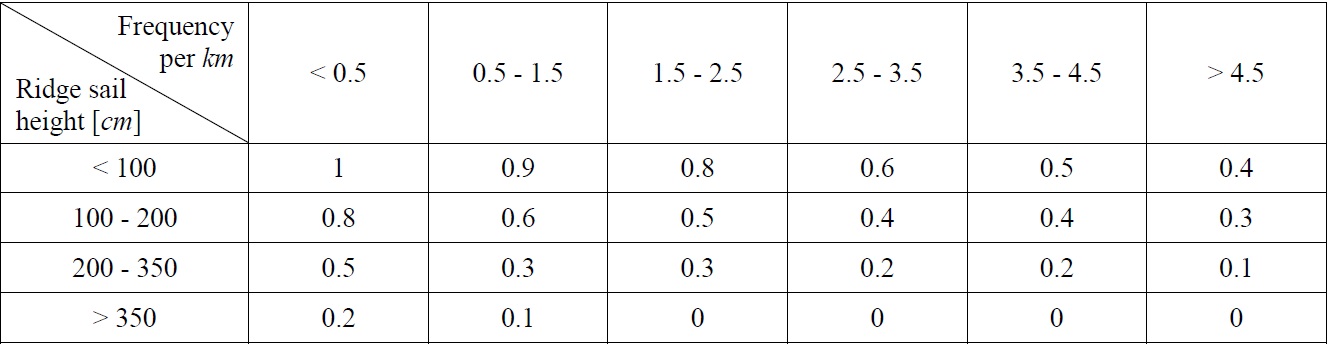
Speed reduction factors for ice ridges.
In open sea where no ice exists, the ship speed is influenced by environmental factors such as current, wave, and wind. Those factors can accelerate or decelerate the ship speed depending on their size and direction. In the head sea where the ship is against external effects, for instance, the speed reduction increases. Summarized speed reductions are shown in Table 4, where BS and Vc stand for the base speed of ship and the current speed, respectively. The ship speed is set to be constant, typically lower than the base speed, where the ice concentration is up to 30%. Their effects, however, are ignored when the ice concentration is more than 30%.
[Table 4] Adjusted speed for wind, wave, and currents [in knots].

Adjusted speed for wind, wave, and currents [in knots].
The final consideration for speed reduction is due to miscellaneous environmental conditions such as fog, icing, snowstorm, or ice compression. These conditions result in little to no visibility, and these effects are hard to quantify. Therefore, they are approximately divided into several groups, and linear-like reductions are applied. Table 5 shows an example of speed reduction made by the existence of fog, icing and snowstorm. Their effects are classified into four levels depending on its density. The speed reduction by ice compression is tabulated in Table 6. The ice compression is a crucial factor in determining ship speed reduction. When assisted by an icebreaker, the channel behind the icebreaker may close quickly depending on the level of ice compression, which makes the vessel harder to navigate. Unfortunately, it is not easy to formulate the effect of ice compression with clean mathematical functions. In our simulation model, the speed reduction is roughly classified into four discrete levels.
[Table 5] Speed reduction factors for fog, icing, and snowstorm.
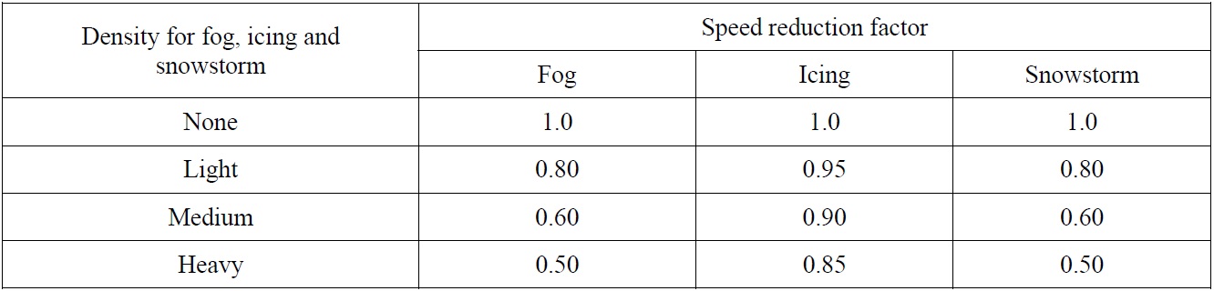
Speed reduction factors for fog, icing, and snowstorm.
[Table 6] Speed reduction factors for ice compression.
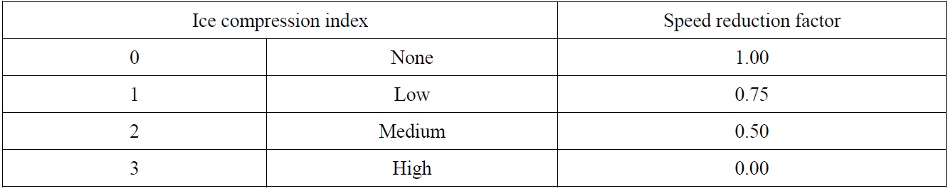
Speed reduction factors for ice compression.
>
Data manipulations for intermediate computing factors
The distance between the origin and destination ports is simply computed by the spherical law of cosines (http://mathworld.wolfram.com/SphericalTrigonometry.html). To verify the accuracy, the results were compared with those of Google Earth and the errors were within 0.22%.
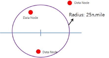
The numerical model uses the curvilinear grid system where two neighboring nodes are normally 26 nautical miles (
>
Input parameters for cost estimation
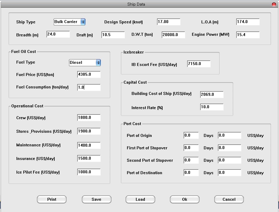
To determine the optimal route, the user starts with the initial dialog shown in Fig. 9. It includes ship data, fuel cost, operational cost, capital cost, and port cost. They differ by ship to ship and season to season. The design speed is an important factor in determining base speed. Water depth of route becomes critical when it is not deep enough to allow the ship’s depth.
The number of stays at origin, stopover, and destination ports affects final voyage hours. Fuel and oil costs, operational costs, capital cost, and port cost must be collected from the providers. The icebreaker may not be used during the voyage but its fee should be known in advance to correctly reflect the potential maximum cost.
Dijkstra's algorithm (Dijkstra, 1959), named after Dutch computer scientist Edsger Dijkstra, was introduced between 1956 and 1959. It was a graph search algorithm aimed at finding the shortest path associated with path costs, producing a shortest path tree. His algorithm has been widely used in routing and graph algorithms. The algorithm is so popular that its concept is available anywhere (Skiena and Revilla, 1999).
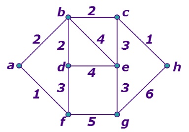
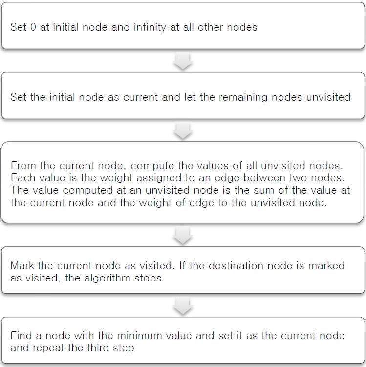
As a way to find an optimal route, Dijkstra suggested the concept of weights between two neighboring nodes. An example of the weighted graph is illustrated in Fig. 10. The values written on edges are the weights that the user wants to optimize. If the values represent the navigating hours, the optimized object is the minimized navigating hour. On the other hand, the weights of cost will yield the least costly route. The procedure of finding an optimized value is summarized in Fig. 11.
To find the secondary optimized route, another algorithm has to be sought. This step can be simply implemented by a slight modification of the original Dijkstra algorithm. Each link between two nodes of the optimal route computed is intentionally blocked and the Dijkstra algorithm is applied. This blocking process is repeated for every link and among all the paths obtained the minimal path is selected as the secondary route. The routes at subsequent levels can be similarly calculated.
The ultimate purpose of the transit simulation is to provide optimal routes prior to real voyage. Verifying the simulated results is an indispensible process, which can be done by applying the algorithm to the cases in which previous navigation records are available. Nonetheless, predicting current or future routes is not an easy task that should be performed with caution as inaccuracy can result in enormous losses. The reliability of the simulation will improve, however, when the simulations are repeatedly carried out and their results are verified with actual data accumulated from real voyage.
The transit model and the algorithm of optimal routes for transit simulation have been implemented and tested in the Arctic region. The simulation is performed by enabling the user to select the months, years, and departing and arriving ports. If multiple years or months are simultaneously selected, their average value at each node is used. The user is responsible for inputting the ship data in advance.
The way that the implemented code works is to simply display the optimal routes based on the user’s input. The calculated routes are displayed on a graphic window and its detailed information is described in a text file that can be separately viewed at any time.
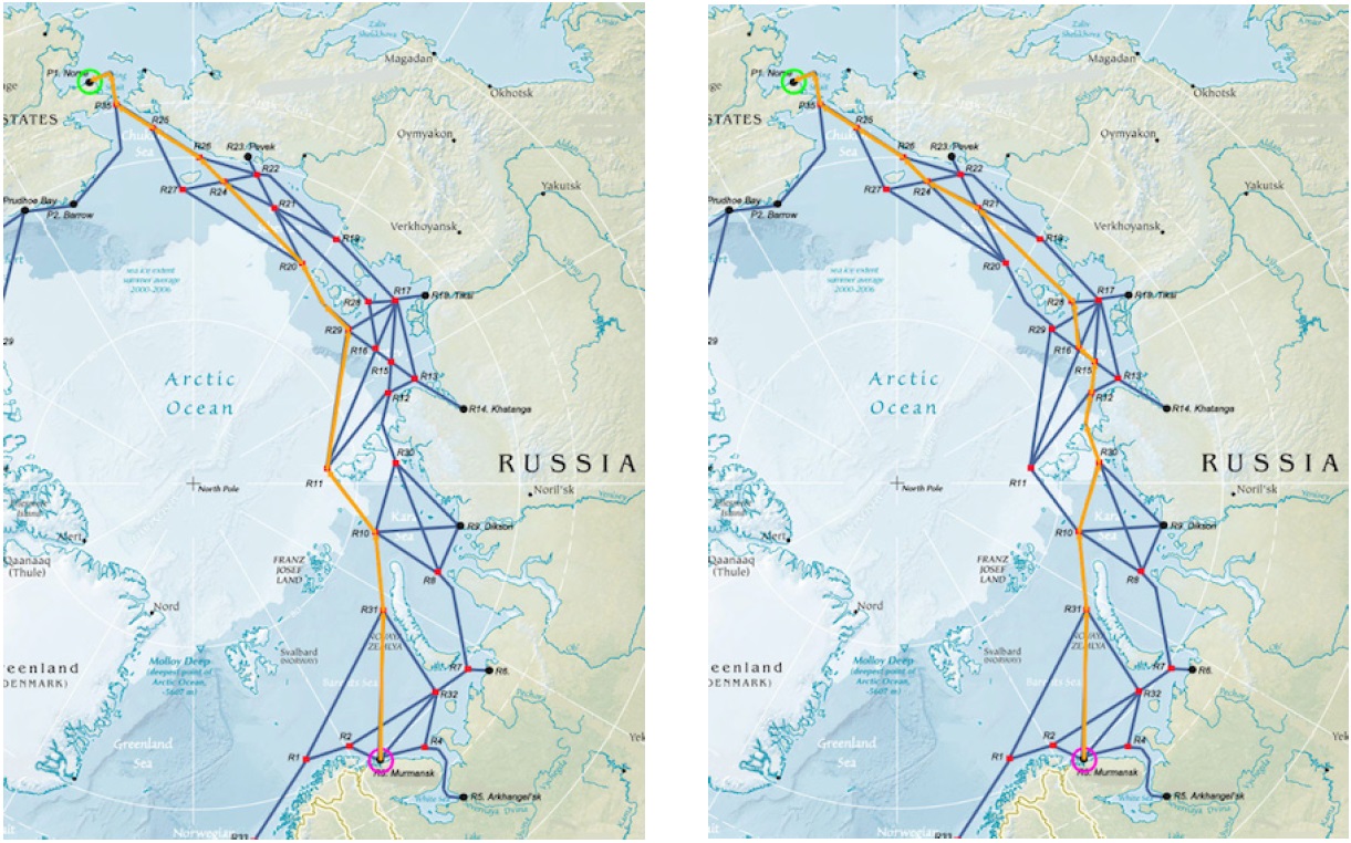
The optimal routes simulated for April and October over the years of 2000 to 2004 are depicted in Fig. 12. The optimal route marked in orange (lighter color) on the map shows the route that offers the fastest transit time, which implies the minimal cost.
The other detailed reports associated with the routes computed are provided to the user, as illustrated in Table 7. Readers are advised to note the subsequent optimal routes are also included in the report. Since the cost associated with the voyage is computed based on ship speed, the travelling distance of a route shown in the map does not have to be the shortest; rather it suggests the spatial trajectory that a ship can take.
The simulation results throughout the four months (January, April, July, and October) during the years 1995-1999 and 2000-2004 are tabulated in Table 8. It is confirmed that the ice condition of the late 90s had extended into the early 2000s, without much change. Since global warming had influenced summer ice conditions since 2006, the aforementioned extension became meaningless following that year. Table 8 demonstrates the similarity of ice conditions between the simulated results of 1995-1999 and those of 2000-2004.
[Table 7] An example of detailed results of an optimal route.
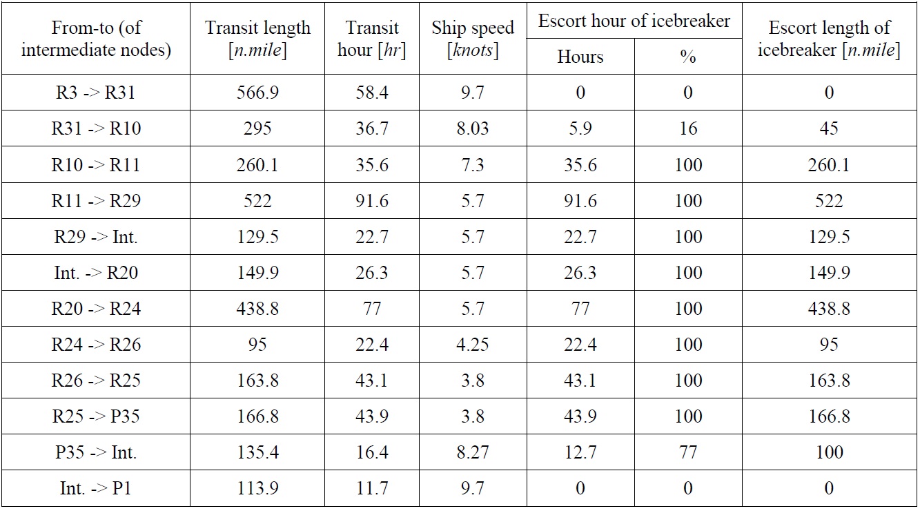
An example of detailed results of an optimal route.
[Table 8] Simulation results during years 1995-1999 and 2000-2004.
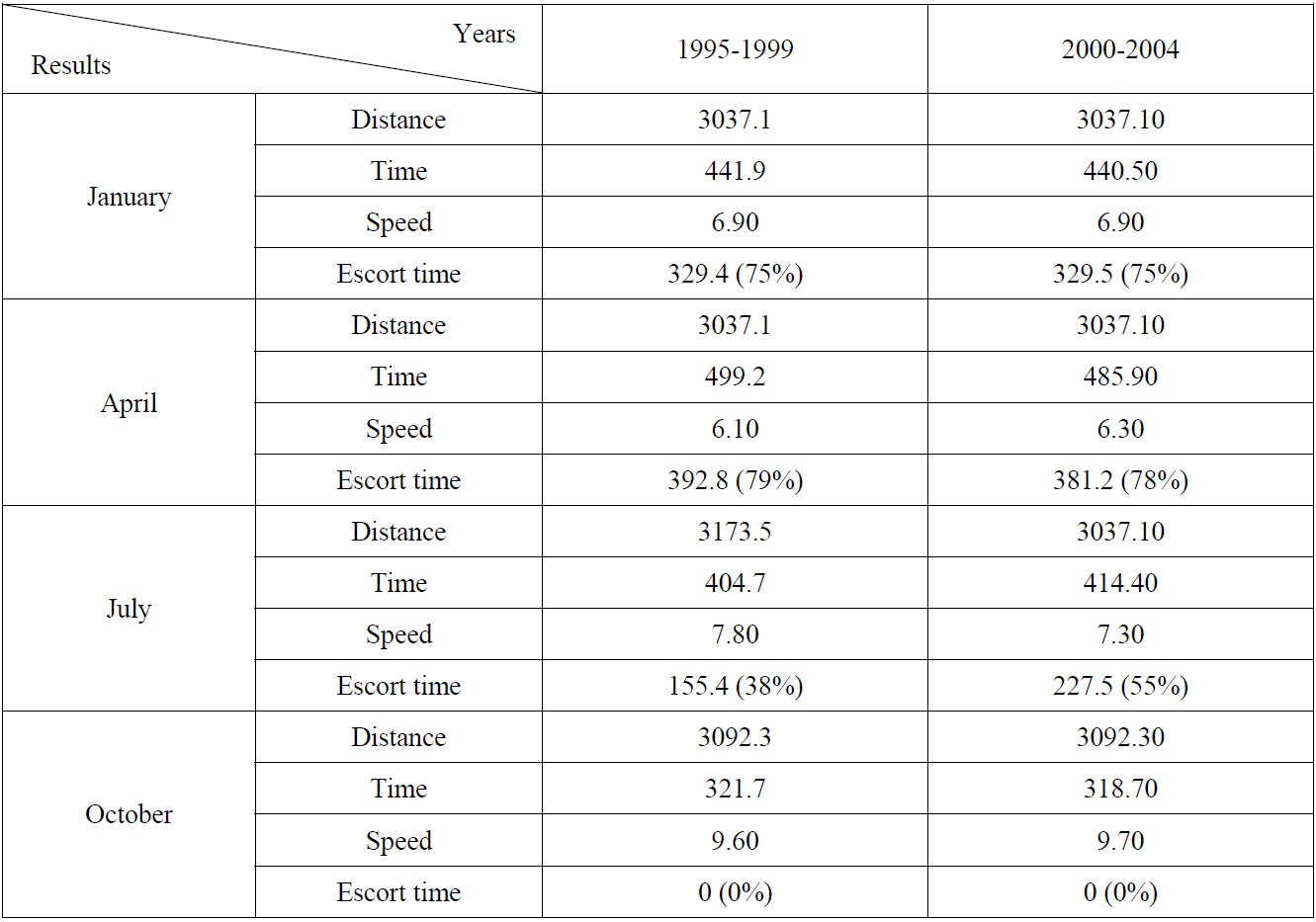
Simulation results during years 1995-1999 and 2000-2004.
>
Comparison with previous models
The simulation results need verification to make sure that the transit model and the associated algorithm are correctly established. If field experiments were performed and their results are available, the comparison of field data with simulated results would be the best option. Unfortunately, those kinds of data are not generally available; hence this option is not realistic. Another option is to compare the simulated results with other ones previously published. However, lack of comparable simulated results in academic literature makes this approach impractical.
A derived way adopted in this work is to indirectly compare the simulation results with the previously released results. However, instead of one-to-one direct comparison of their results, the focus is the confirmation of tendency of those results. Two official results released by CRREL and INSROP are considered. The two research groups performed transit simulations based on the ice and environmental data established in the 1990s (Mulherin et al., 1996; Lysaker, 1999). Even though they did not release every piece of information, some useful results were still available. The comparison between the simulated results by the model introduced in this work and those of CRREL is summarized in Table 9.
[Table 9] Comparison between simulated and CRREL models.
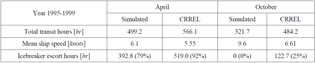
Comparison between simulated and CRREL models.
The table above indicates that direct comparison can hardly demonstrate one-to-one relation between the two results, as expected. In each season, however, the numbers between the two models exhibit relative association, which may be regarded as an affirmative aspect.
There may be several reasons for the differences in numbers. The primary factor lies in the difference of ice and environmental data, as the determination of routes is completely dependent on the data. Among the data, the most influential factor assumed in this work is the existence and size of ice ridges.
Ridges are a critical component that slows down the icebreaking vessels. Sometimes the ships take a detour due to heavy ridges. Unfortunately, the exact distribution of ridge’s sail height or spacing is not precisely known, unlike the other factors such as ice thickness or sea ice concentration. The distribution of averaged ridge’s sail height published by Riska and Salmera (1994) is a useful source available to the public, but further research or updated results remain unknown to us. It can be deduced that CRREL included the effect of ice ridges, which slows down the ship speed. On the other hand, the simulated model that does not consider ridges yields the faster speed.
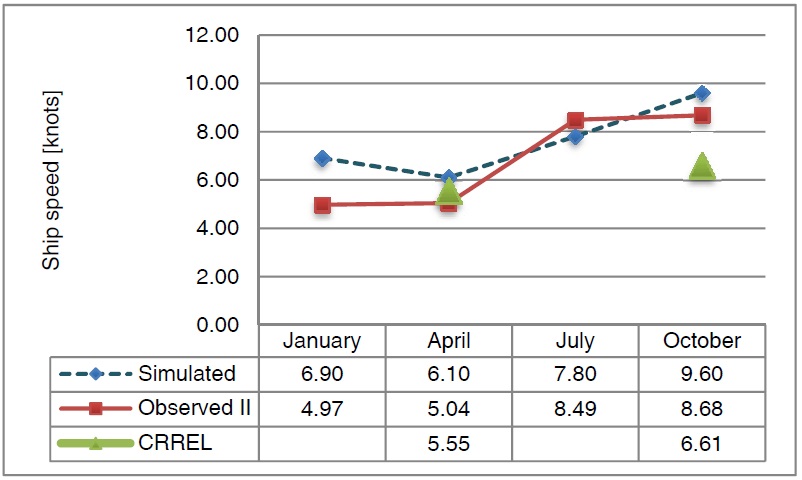
Fig. 13 compares the ship speeds obtained from three different methods. Observed II is another simulated result using the observed data previously published by the authors (Choi et al., 2010). In CRREL’s report, April, June, August, and October’s speeds are available; thus only two months’ (April and October) results are included in the figure. Simulated is the result computed using the algorithm introduced in this work.
In CRREL’s model, the speed in October is far slower than those of other two transit models. This discrepancy is generally attributed to the existence of ridges. The previous results marked as Observed II indicate that the ship speed varies depending on two extreme seasons, summer and winter. The simulated model yields more reasonable speed variation. The ship speed becomes the minimum in April when the Arctic area is experiencing heavy ice and severe weather conditions. The speed gets faster as the ice is melting in summer and fall and becomes slow in winter. It is obvious that the ship speed would be lowered if ridges were included in the model.
As no experimental results of real voyage are available, it is not appropriate to judge which model is accurate and which is not. Nevertheless, the new model, based on the numerical simulation, will produce more reliable results with the feedback from computation or the consistent comparison with field experiments.
An improved algorithm to calculate the optimal Arctic routes has been introduced. The transit model uses ice and environmental data by analyzing an ice model numerically modeled. Even though the simulated results do not perfectly match with those obtained from the observed data, the newly developed algorithm offers an elegant and analytic way to predict routes in coming years. In fact, it is difficult to tell which result closely matches the real situation, partly due to the rare availability of observed data.
One of the difficulties confronted in the simulation is the existence of ridges. The numerical model cannot precisely deal with ridges in its governing equation in the current version and thus the ridge data are not included in the model. We cautiously conclude the model used in this work yields the shorter navigation hours than the previous results owing to the ridge-free condition. Therefore, knowing the exact distribution of ridges will be essential in future research.
Another difficulty is to consider the effect of ice compression. In the current simulation model, four discrete levels are used to determine the speed reduction by the ice compression. This reduction factor needs further investigation.
The developed algorithm will be used as a transit guide in the Arctic region. Its contribution to the optimal route simulation will be significant as the reliability of the sea ice model improves after feedback and correction.
Future work includes the improvement of strategy in finding an optimal route. Instead of inserting equidistant and imaginary nodes that are linearly interpolated by two neighboring nodes, the strategy is to let the route follow the denser nodes offered by a refined sea ice model. This approach is currently under development.


![Adjusted speed for thickness and concentration of ice [in knots].](http://oak.go.kr/repository/journal/12408/E1JSE6_2013_v5n2_210_t002.jpg)

![Adjusted speed for wind, wave, and currents [in knots].](http://oak.go.kr/repository/journal/12408/E1JSE6_2013_v5n2_210_t004.jpg)