Gk Production of turbulent kinetic energy [kg/ms3]
I Unit tensor [-]
k Turbulent kinetic energy [m2/s2]
P Pressure [Pa]
p Estimated order of accuracy of the computational method [-]
RE Richardson extrapolated value [-]
Re Reynolds number [-]
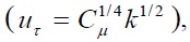
uτ Friction velocity [m/s]
U∞ Free stream velocity [m/s]

Velocity vector [m/s]
yp Distance from wall to cell center [m]
ε Turbulent dissipation rate [m2/s3]
μ Viscosity [kg/m-s]
μeff Effective viscosity [kg/m-s]
μt Turbulent viscosity [kg/m-s]
νt Turbulent eddy viscosity [m2/s]
ρ Density [kg/m3]
κ Surface roughness [-]

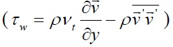
Turbulent stress tensor [Pa]
τw Wall shear stress [Pa]
φ Computational solution variable for uncertainty assessment [-]
With the rapid development of CFD techniques, computational analyses complement experiments in many parts of the hullform design. Korea Ocean Research and Development Institute (KORDI) developed a CFD code for the prediction of ship resistance and propulsion performances (Kim et al., 2002). Many shipbuilding companies in Korea adopted the code as their CFD tool for hull form development. FLOWTECH also developed a CFD code for ship resistance performance prediction (Leer-Andersen and Larsson, 2003). General purpose CFD codes, such as FLUENT, STAR-CCM+, and CFX, are also used in shipbuilding companies, research institutes, and universities (Rhee et al., 2005; Rhee, 2009; Park and Chun, 2009; Choi et al., 2010; Seo et al., 2010, Park et al., 2010). Specialized CFD codes for hull form development, such as the ones developed by KORDI and FLOWTECH, are equipped with limited computational methods and their applications are limited to common ship hull shapes. On the other hand, general purpose CFD codes can handle non-conventional ships and provide various computational methods. However, their purchase and maintenance prices are quite high. Especially, annual licensing fee for parallel computing is another burden. Due to these reasons, interest in free CFD codes has increased recently. Among free CFD codes, Open FOAM, which is an object-oriented, open source CFD tool kit draws huge interest recently (Jasak, 2009).
Many CFD codes and libraries have been developed using the OpenFOAM platform. Favero et al. (2009) developed a new tool for CFD simulation of viscoelastic fluids. Kunkelmann and Stephan (2009) implemented and validated a nucleate boiling model using OpenFOAM platform. Bensow and Bark (2010) employed an approach to simulate dynamic cavitation behavior based on the large eddy simulation, using an implicit approach for the subgrid terms and applied to a propeller flow. Kissling et al. (2010) developed a coupled pressure based solution algorithm to model interface capturing problems for multiphase flows. Silva and Lage (2011) coupled a multiphase flow formulation with the population balance equation solution by the direct quadrature method of moments. Dittmar and Ehrhard (2011) developed a phase change model library including the contact line evaporation model and on the conjugate heat transfer between solid and fluid. Petit et al. (2011) investigated the swirling flow with helical vortex breakdown in a conical diffuser. Park and Rhee (2012, 2013) developed a CFD code (SNUFOAM-Cavitation) and applied it to super- and cloud cavitations. Many researchers have developed new libraries and CFD codes for their purpose. However, studies on free CFD codes in ship hydrodynamics are yet to be reported, even though the dependency for commercial CFD codes have been intensified over many years.
Therefore, in the present study, a Reynolds-averaged Navier-Stokes (RANS) equations solver that couples the velocity and pressure was developed based on a cell-centered finite volume method. The developed CFD code, termed SNUFOAM, was based on the OpenFOAM (Jasak, 2009), and the authors implemented wall function (Launder and Spalding, 1972) library.
The present study focused on the turbulent flow around a surface ship. The objectives were therefore (1) to develop and validate SNUFOAM, and (2) to understand the turbulent flow around a surface ship by comparing the results with a comercial CFD code.
The paper is organized as follows. The description of the physical problem is presented first, and this is followed by the computational methods. The computational results are then presented and discussed. Finally, a summary and conclusions are provided.
The equations for the mass and momentum conservation were solved to obtain the velocity and pressure fields. The equation for the conservation of mass, or the continuity equation, can be written as

where
is the velocity vector.
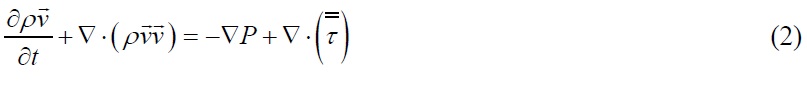
The equation for the conservation of momentum can be written as
where
), is given by

with the second term on the right-hand side representing the volume dilation effect, where
Once the Reynolds averaging approach for turbulence modeling is applied, the unknown term, i.e., the Reynolds stress term, is related to the mean velocity gradients by the Boussinesq hypothesis, as follows

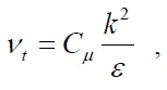
The standard


where
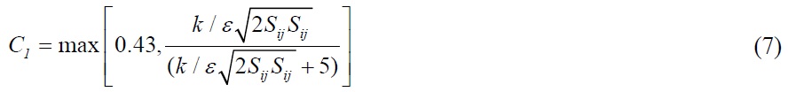
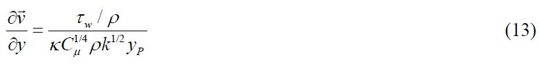
The turbulent viscosity was used to calculate the Reynolds stresses to close the momentum equations. The wall function was used for the near-wall treatment (Pope, 2000; Launder and Spalding, 1972). A detailed description of the wall functions is as followed.
From the assumption of the equilibrium state (
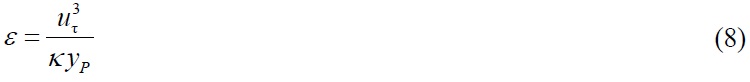
where
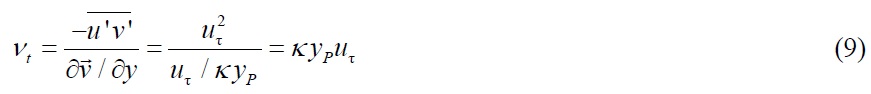
and
which leads to the expression for

From the definition of
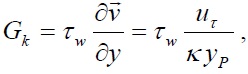
the formulation of the production of turbulent kinetic energy in the turbulent kinetic energy equation, proposed by Pope (2000), is expressed, as follows
where
The wall shear stress of the log-law is commonly obtained (Launder and Spalding, 1972; Craft et al., 2002).

Thus,
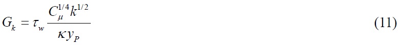
From the definition of
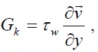
the formulation of the production of turbulent kinetic energy in the turbulent kinetic energy equation, proposed by Launder and Spalding (1972), is expressed, as follows
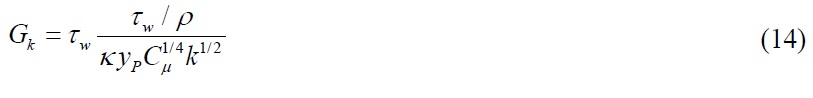
The CFD code including the equation (14) was named SNUFOAM-WF2.
A pressure-based cell-centered finite volume method was employed along with a linear reconstruction scheme that allows the use of computational cells of arbitrary shapes. The solution gradients at the cell centers were evaluated by the least-square method. The convection terms were discretized using the van Leer scheme (van Leer, 1979), and for the diffusion terms, a central differencing scheme was used. The velocity-pressure coupling and overall solution procedure were based on a pressure-implicit with splitting order (PISO) type segregated algorithm (Issa, 1985) adapted to an unstructured grid. The discretized algebraic equations were solved using a pointwise Gauss-Seidel iterative algorithm, while an algebraic multi-grid method was employed to accelerate solution convergence.
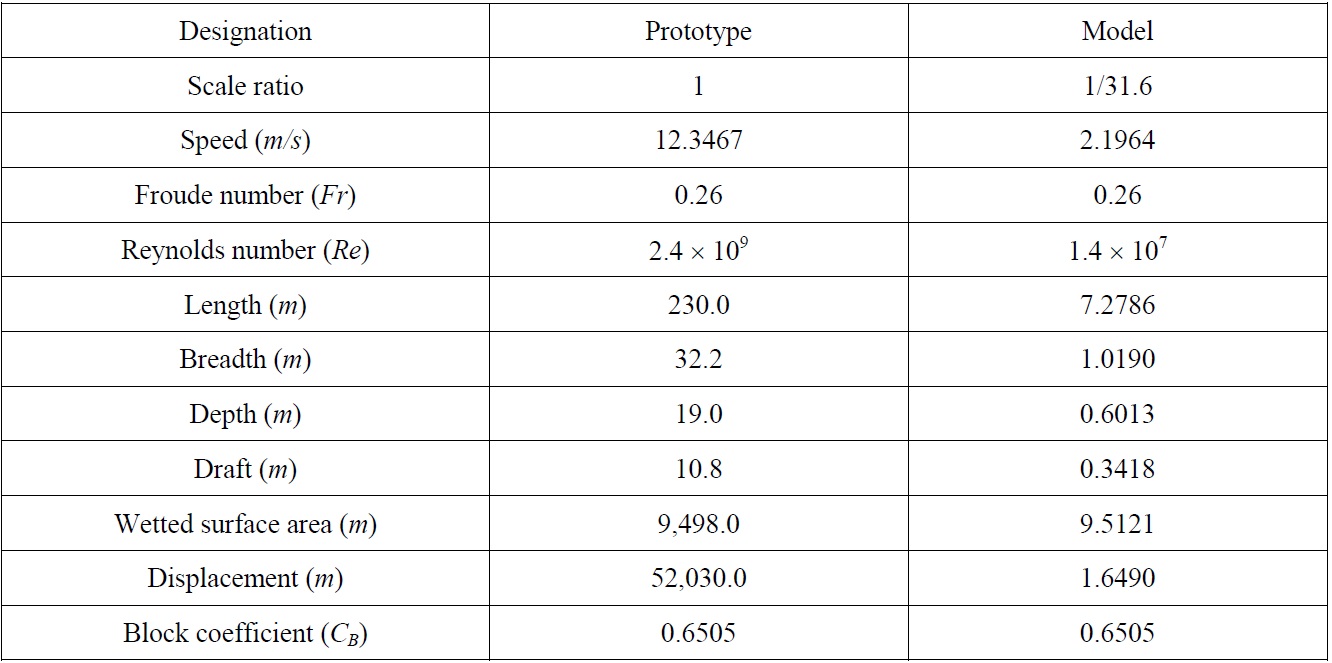
KRISO container ship (KCS), a 3,600
[Table 1] Principal particulars of KCS.

Principal particulars of KCS.
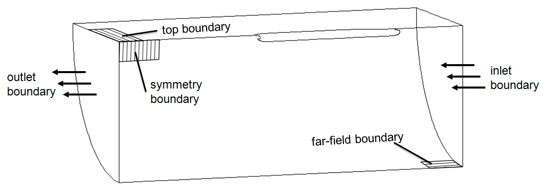
In the Cartesian coordinate system adopted here, the positive
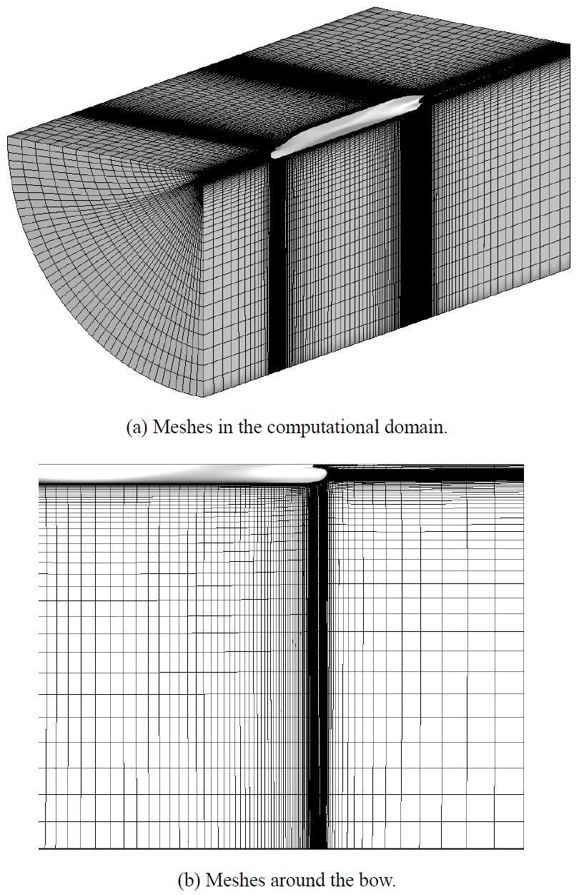
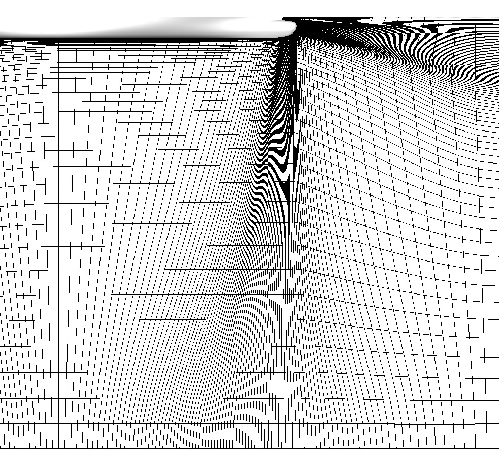
The mesh generation was carried out using Gridgen V15.17, commercially available software. A single-block mesh of 370,000 hexahedral cells was used as shown in Fig. 3. Along the length of the ship, 180 cells were used, while along the girth of the ship, 45 cells were applied.
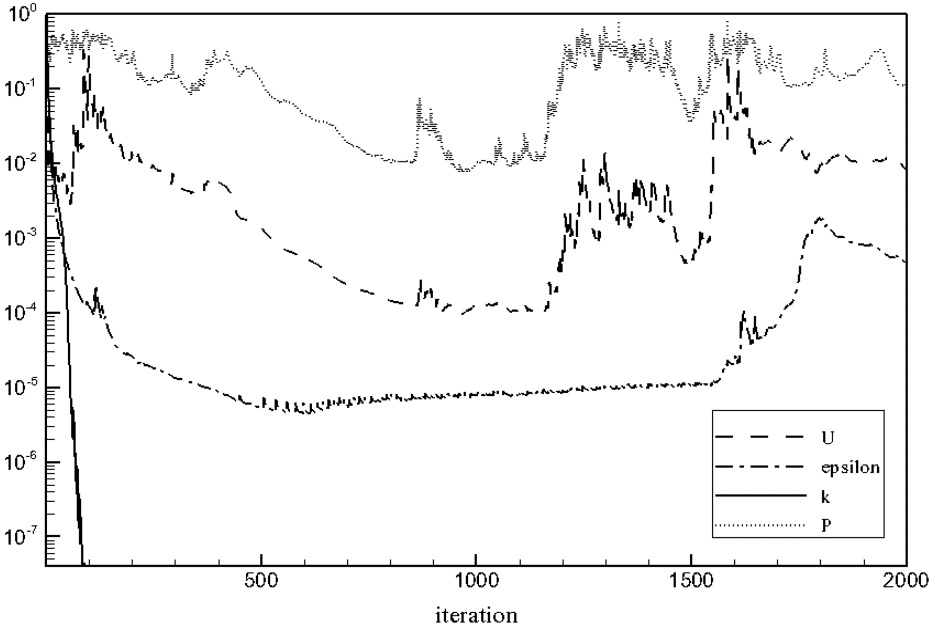
To evaluate the numerical uncertainty in the computational results, the concept of the grid convergence index (GCI) was adopted. Three levels of mesh resolution were considered for the solution convergence of the resistance coefficient (C
The order of accuracy can be estimated as
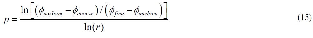
where
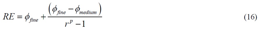

where
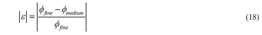
and where
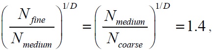
with the cell count,
[Table 2] Numerical uncertainty assessment.
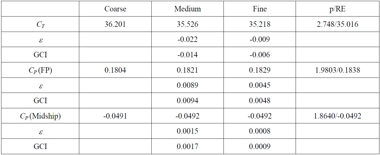
Numerical uncertainty assessment.
Steady computations were done for the Reynolds number (based on
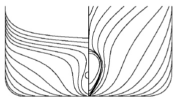
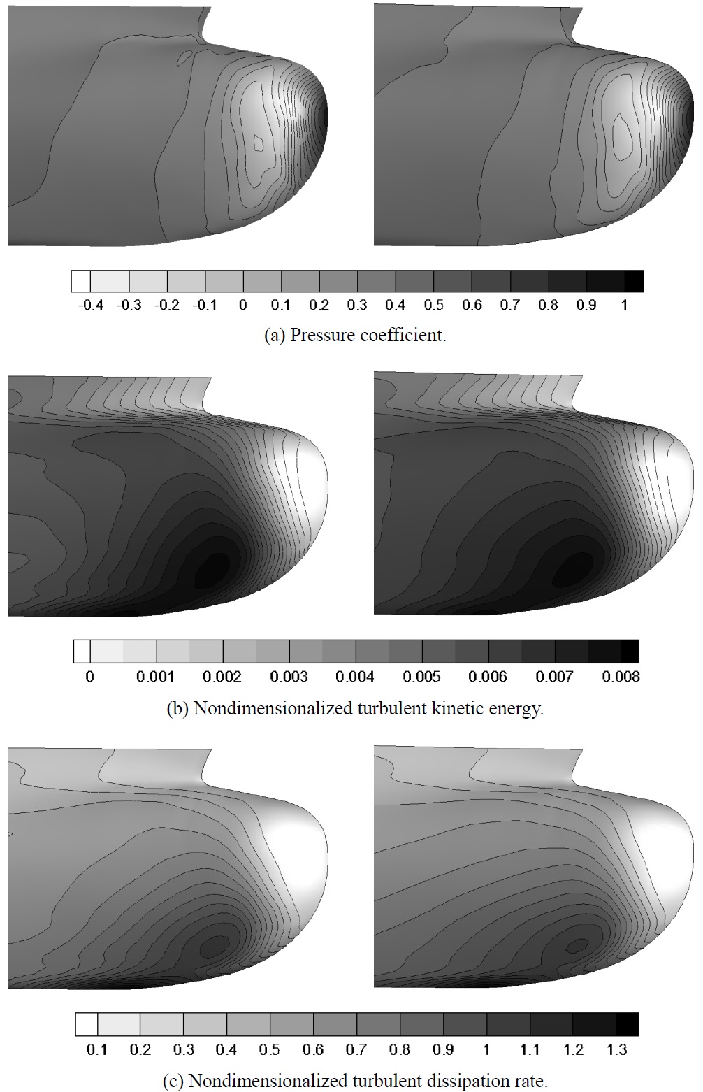
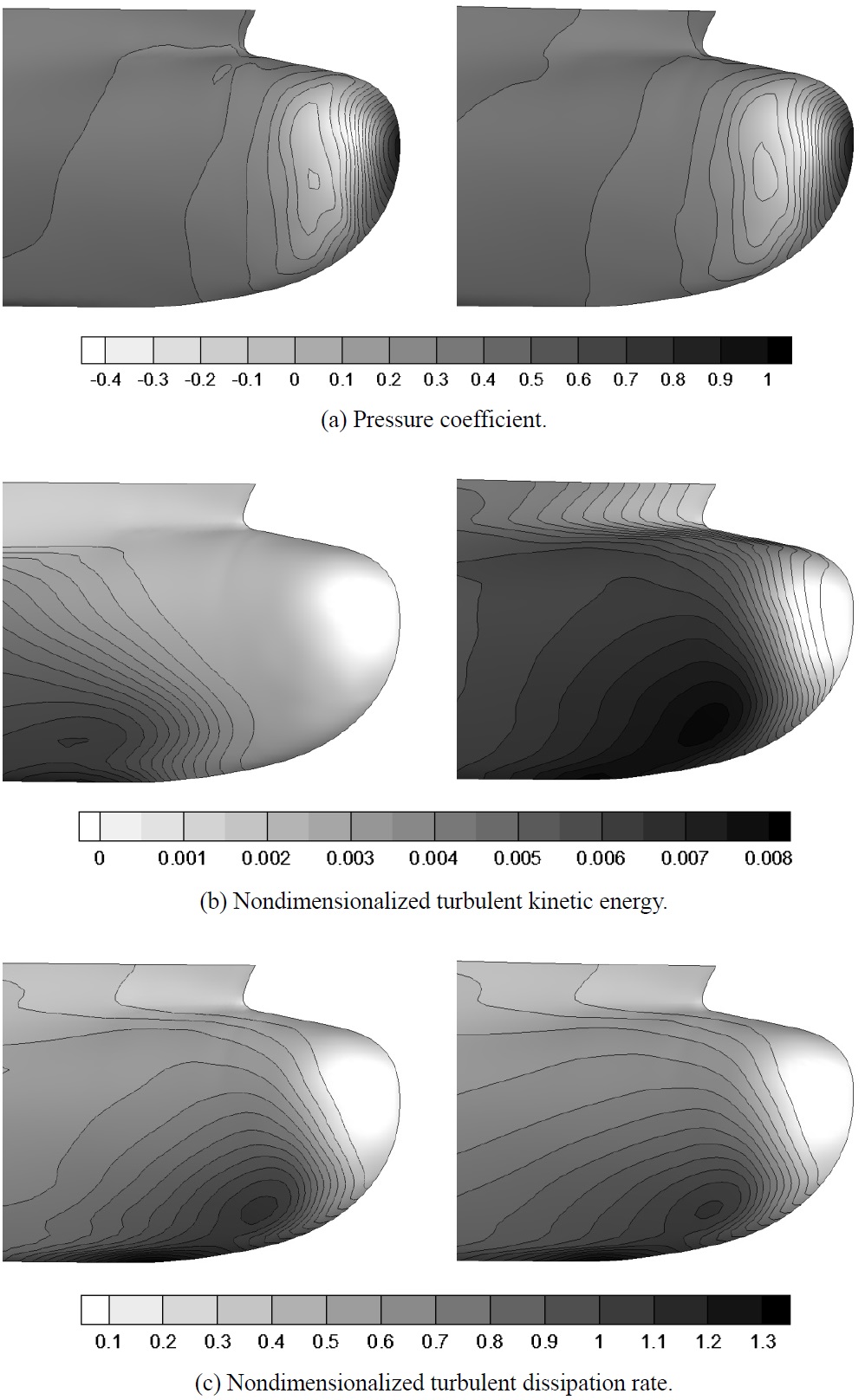
Firstly, computations were done with the new mesh using SNUFOAM-WF1. The validation of SNUFOAM was conducted by comparing with the results of a commercial CFD code, FLUENT, which showed good results in ship hydrodynamics (Rhee et al., 2005; Rhee, 2009; Park and Chun, 2009; Choi et al., 2010; Seo et al., 2010). Fig. 8 shows the pressure coefficient, nondimensionalized turbulent kinetic energy (
The same flow was also simulated using SNUFOAM-WF2, which did not include the assumption of the equilibrium state. The equation (14) was calculated by substituting the friction velocity
which was derived from the assumption of the equilibrium state, to the equation (11). Fig. 9 shows the pressure coefficient, nondimensionalized turbulent kinetic energy, and nondimensionalized turbulent dissipation rate contours around the bow. The nondimensionalized turbulent kinetic energy and nondimensionalized turbulent dissipation rate computed using SNUFOAM-WF2 showed the nearly same development with those computed using FLUENT. The wall function (Launder and Spalding, 1972), which did not include the assumption of the equilibrium state, improved the turbulence development around the bow. Thus the turbulent production was larger than the turbulent dissipation in the bow region. Another reason could be numerical errors. The velocity gradient, which was related with the wall shear stress
plays an important role here. Equation (14) includes the velocity gradient twice, while Equation (11) includes the velocity gradient only once.
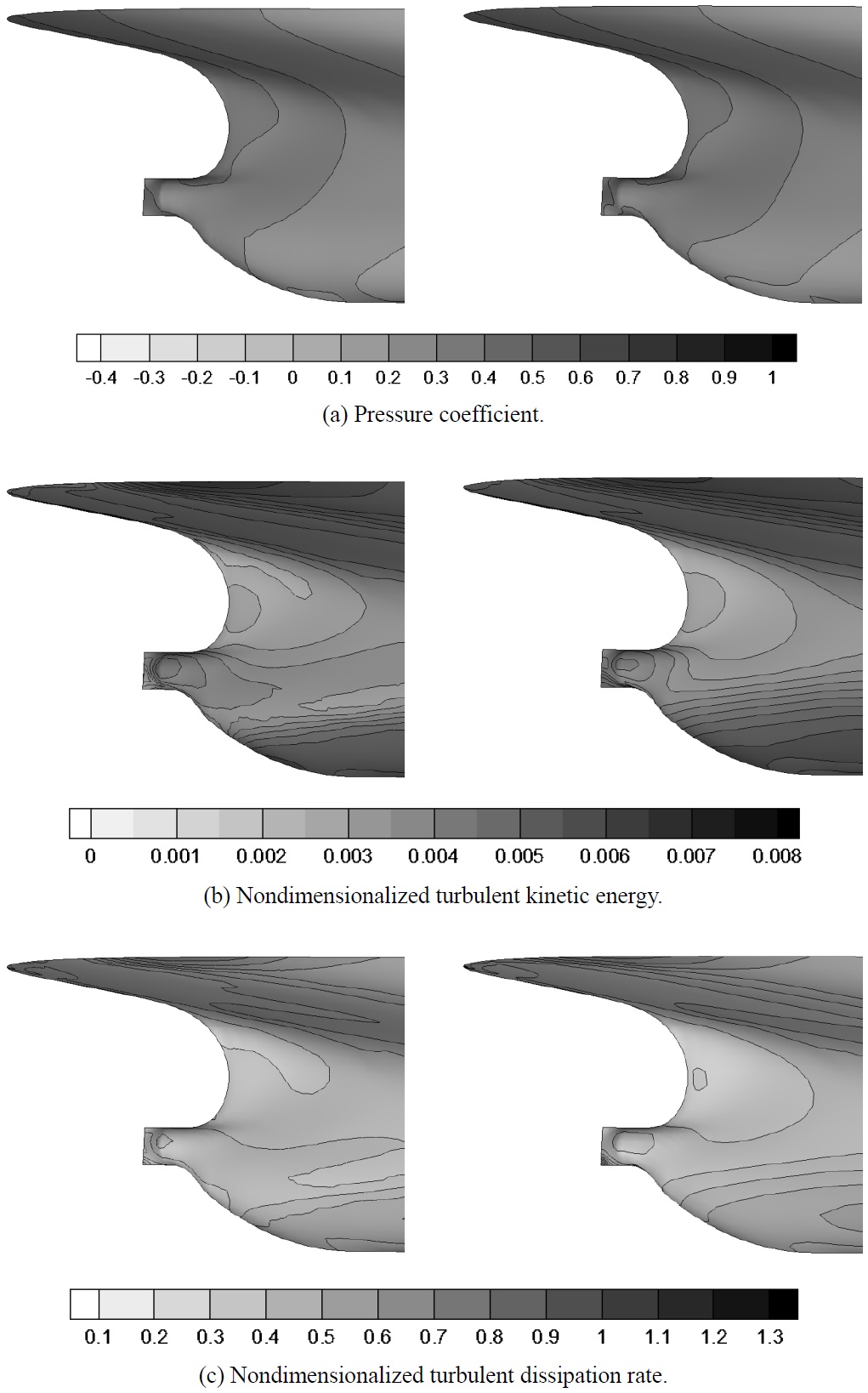
Fig. 10 shows the pressure coefficient, nondimensionalized turbulent kinetic energy, and nondimensionalized turbulent dissipation rate contours around the stern. The pressure coefficient, nondimensionalized turbulent kinetic energy, and nondimensionalized turbulent dissipation rate contours computed using SNUFOAM-WF2 showed quite close to the results computed using FLUENT.
A CFD code was developed using the OpenFOAM (Jasak, 2009), and the authors implemented wall function (Launder and Spalding, 1972) library. The mesh sensitivity was evaluated for the skewness and aspect ratio of the cells. SNUFOAM showed good convergence with low aspect ratio cells. The results computed using SNUFOAM-WF1 needed the long entrance length for the development of the turbulent boundary layer in the bow, and was different from those computed using FLUENT. SNUFOAM- WF2 was developed including another wall function, which did not include the assumption of the equilibrium state between the turbulent kinetic energy and turbulent dissipation rate in the log law layer. The results computed using SNUFOAMWF2 showed quite close to those computed using FLUENT. It is expected that SNUFOAM including the volume fraction transport equation (Park and Rhee, 2011) can substitute a commercial CFD code for the prediction of ship resistance performance in ship hydrodynamics.