In the early 1980s, attention focused on the possibility that PTS events could challenge the integrity of the RPV because operational experience suggested that overcooling events, while not common, did occur, and because the results of in-reactor materials surveillance programs showed that US RPV steels and welds, particularly those having high copper content, experience a loss of toughness with time due to neutron irradiation embrittlement. These recognitions motivated analysis of PTS and the development of toughness limits for safe operation. It is now widely recognized that state of knowledge and data limitations from this time necessitated conservative treatment of several key parameters and models used in the probabilistic calculations that provided the technical basis [1] of the PTS Rule [2]. To remove the unnecessary burden imposed by these conservatisms, and to improve the staff’s efficiency in processing exemption and license exemption requests, the NRC undertook the PTS re-evaluation project [3,4].
The PTS re-evaluation project was conducted between 1998 and 2009 by the United States Nuclear Regulatory Commission USNRC. Assistance and data was provided by the commercial nuclear power industry operating under the auspices of the Electric Power Research Institute (Electric Power Research Institute). Toward the end of this time the project findings were reviewed by the Advisory Committee on Reactor Safeguards (ACRS), the Nuclear Energy Institute (NEI), the public, and a panel of national and international experts. These reviews provided the basis for numerous model corrections and improvements. Based on the findings of this project, the NRC initiated rulemaking on a voluntary alternate to 10 CFR 50.61 in 2006 [5,6]. Rulemaking was completed on January 4, 2010 when 10 CFR 50.61a was published in the Federal Register [7].
This description of the PTS re-evaluation project begins in Section 2 with a discussion of the risk limits that provide the basis for the embrittlement-based screening limits adopted in 10 CFR 50.61a. Then Section 3 describes the probabilistic model that was used to develop relationships between risk limits and embrittlement limits. Section 4 describes the results obtained from this model, and Section 5 describes how they were used to establish regulatory limits for 10 CFR 50.61a. Section 6 compares the regulatory provisions of 10 CFR 50.61 and to 10 CFR 50.61a.
In the Atomic Energy Act of 1954, which allowed the first large scale commercial use of nuclear energy in the United States, the United States Congress instructed the Atomic Energy Commission (AEC, the precursor to the NRC) to “
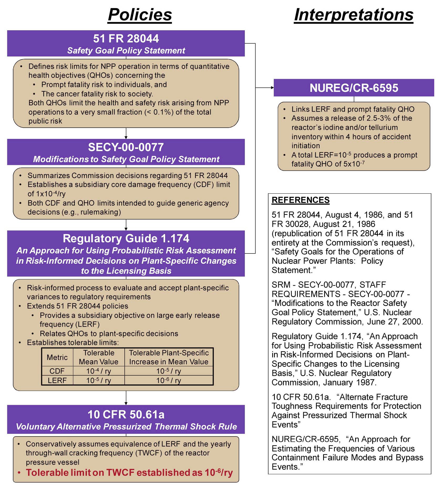
The work on safety goals begun after the Three Mile Island accident culminated in the issuance of a safety goal policy statement in 1986 [11]. This statement, along with other policies that lead the way to the risk limits adopted in the PTS re-evaluation project, are illustrated in Fig. 1. Key points that link the PTS risk limits to Commission policy may be summarized as follows. The 1986 safety goal policy statement defines risk limits for plant operation in terms of quantitative health objectives (QHOs) that measure the prompt fatality risk to individuals, and the latent cancer fatality risk to society [11]. The QHOs for both limit the health and safety risk arising from nuclear plant operations to a very small fraction (< 0.1%) of the total public risk. In 2000, the 1986 policy statement was modified to include a subsidiary limit on the core damage frequency (CDF) of 1x10⁻⁴/ry, and was clarified by stating that both the CDF and QHO limits were intended to guide generic agency decisions (e.g., rulemaking) [12]. The information in both policy statements was incorporated into, and augmented by, the publication of Regulatory Guide 1.154 [13]. This guide provided yet another subsidiary goal, the large early release frequency (LERF). RG1.154 also defined limits on the total CDF and LERF, as well as on the CDF and LERF seen to arise from any single cause (see the table in Fig. 1). Finally, this ΔLERF limit of 10-6/ry was used in the PTS re-evaluation project to establish a limit on the through-wall
cracking frequency (TWCF) of 10-6 events per reactor operating year. The TWCF limit is based on a conservatively assumed equivalence between TWCF and LERF [3].
Beyond the considerations that led to the 10-6 limit, the staff also considered the definition of vessel “failure.” Failure was defined as the initiation of a rapidly propagating fracture from a pre-existing flaw in the vessel beltline region, followed by sufficient extension of that flaw to penetrate fully the thickness of the RPV wall. This definition was adopted because through-wall cracking of the RPV was viewed as a measure closely related to the potentially significant public health consequences that are discussed in Commission policy guidance. An assessment of the sequence of events between vessel “failure” and either core damage or LERF revealed that LERF is an unlikely consequence of through-wall cracking in the overwhelming majority of scenarios, thereby validating the conservatism of assuming that LERF=TWCF for the purpose of associating reference temperature based screening metrics with a numeric risk limit.
3. TECHNICAL MODEL / METHODOLOGY
Fig. 2 illustrates our overall model of PTS, which involves three major components:
1. Probabilistic Evaluation of Through-Wall Cracking Frequency: Estimates the frequency of through-wall
cracking due to a PTS event.
2. Acceptance Criterion for Through-Wall Cracking Frequency: Establishes a value of reactor vessel failure frequency based on NRC guidance on riskinformed decision-making.
3. Screening Limit Development: Compares the results of the two preceding steps to determine if a materia property-based PTS screening limit can be established.
Component 2 was described in Section 2 while Component 3 will be described in Section 5. The information provided in this section describes the approach taken to estimate the TWCF (Component 1).
As illustrated in Fig. 2, three main models (shown as solid blue squares) permit estimation of the annual frequency of through-wall cracking in an RPV. First, a
Detailed analyses were performed for three operating PWRs: Oconee Unit 1, Beaver Valley Unit 1, and Palisades to sample a range of design and construction methods. Since this study aimed to develop PTS screening limits applicable to all PWRs in the USA, we needed to understand the extent to which these analyses cover the range of conditions experienced by US PWRs in general. To achieve this goal, we performed sensitivity studies on the TH and PFM models to determine the effect, if any, of credible changes to the models and/or their input parameters on the calculated results. Also, we examined plant design and operational characteristics of five additional plants to determine whether the features identified as being important to our three detailed analyses also characterize the fleet. Finally, in our three detailed analyses we assumed that the only possible origins of PTS events are caused by events internal to the plant. However external events (e.g., fires, floods, and earthquakes) may also be PTS precursors. We therefore examined the potential for external events to produce significant additional risk.
3.2 Probabilistic Risk Assessment and Human Reliability Analysis
3.2.1 Identification and Modeling of Event Sequences (Binning)
The format, structure, and details considered in the current analyses draw considerably from the earlier PRA analyses of PTS [14-17]. In addition to recognition of the results and the reasons for the results from these past analyses, limitations and conservatism associated with the past studies were identified and, to the greatest possible extent, alleviated. Other improvements were adopted with the intent of increasing both the accuracy and comprehensiveness of the PRA representations of the plants. Table 1 summarizes the differences between the current PRA and that used to support the 10 CFR 50.61. Since these improvements were made with the intent of increasing both the accuracy and comprehensiveness of the PRA representations of the plants, they neither systematically increase nor reduce the estimated risk from PTS.
Review of past PRA analyses of PTS provided information on the following four areas:
Identifying the types of sequences that needed to be included in the PRA: These sequences included overcooling scenarios at both full-power operation and under hot-shutdown (HZP) conditions, loss of RCS pressure scenarios, late repressurization scenarios, and scenarios that provide immediate overcooling, as well as those that begin as loss-of-cooling scenarios (i.e., undercooling) and subsequently become overcooling scenarios.
Identifying what types of initiating events needed to be included: These events included small-, medium-, and large-break LOCAs, reactor-turbine trip, loss of main feedwater, loss of main condenser, loss of offsite power (including station blackout), loss of support systems (such as AC or DC buses), loss of instrument air, loss of various cooling water systems, steam generator tube rupture (SGTR), and small and large steam line breaks with and without subsequent isolation.
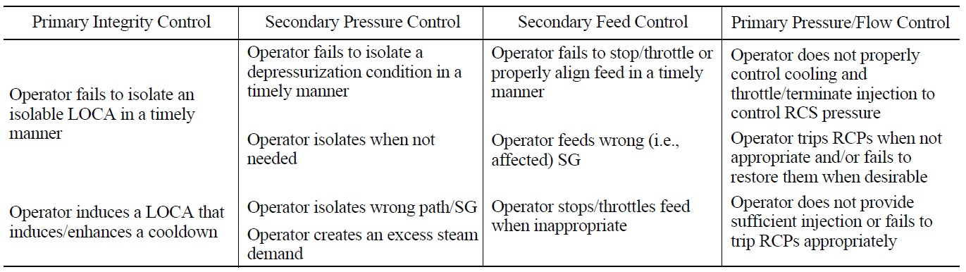
Identifying what functions and equipment status needed to be included: The event trees in the PRA models that depict potential overcooling sequences are based on the status and interactions of four plant functions (i.e., primary integrity, secondary pressure, secondary feed, and primary flow/ pressure) and associated plant equipment. In the plant event trees, the status of equipment relevant to each function is modeled in each PRA.
Identifying what human actions needed to be considered: The process to identify, model, and probabilistically quantify human factors derives largely from NUREG-1624, Revision 1 [18], which uses an expert elicitation approach. In this study, the experts considered both errors of omission and acts of commission. This process identified several general classes of human failures (see Table 2), which have been incorporated into the PRA models.
The event tree-fault tree PRA methodology was used [19]. The modeling approach varied somewhat from plantto- plant because of the order in which the plants were analyzed. Lessons learned in the Oconee analysis impacted
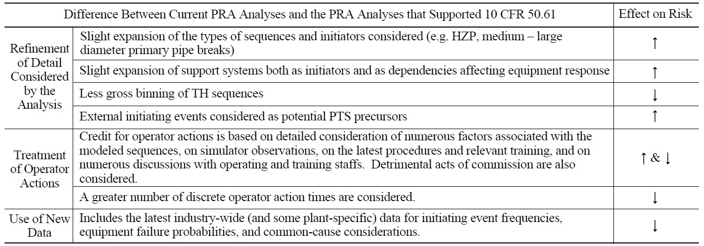
Comparison of PRA Analyses used in this Study with the PRA Analyses that Supported 10 CFR 50.61
[Table 2.] General Classes of Human Failures Considered in the PTS Analyses
General Classes of Human Failures Considered in the PTS Analyses
the Beaver Valley and Palisades modeling approach, for example. Additionally, the availability of information from TH and PFM at the time PRA modeling was performed influenced how the PRA model evolved. For Oconee, initial bins were constructed by developing event tree partitioning rules in SAPHIRE, and then applying those rules to produce the TH bins. Development of the partitioning rules required the analysts to examine the TH information available from preliminary analyses to identify the characteristics that would be important to the binning process. Using this information, the analysts then made judgments as to whether existing TH characteristics could be used to represent new groups of sequences. If the analysts judged that existing characteristics were appropriate (i.e., matched or were more severe than the sequence considered), the uniquely defining characteristics associated with the existing TH analyses were written in rule form for application in SAPHIRE. For those cases where the analysts were sufficiently unsure as to the appropriateness of using existing characteristics the TH analysis being considered formed the basis for a new bin. This iterative process continued until all accident sequence cut sets were associated with a specific TH bin. Once all cut sets were gathered into the initial TH bins, the bins were re-quantified using a truncation limit of 10-10/yr. For Beaver Valley and for Palisades essentially the same process was followed except that knowledge about what was not important in the Oconee analysis was used to limit the detail needed in the models.
With preliminary results available, reviews were conducted to determine whether inaccuracies existed in the models, whether additional potential PTS sequences needed to be modeled, whether additional TH bins should be created to reduce unnecessary conservatism, which human actions were associated with the important TH bins, and which of those human actions should be reexamined to produce even more realistic HEPs.
3.2.2 Uncertainty Quantification
The PRA analysis estimates frequencies of the set of representative plant responses to plant upsets (i.e., scenarios). The major area of uncertainty associated with these frequencies depends on the following factors:
Modeling of the representative plant scenarios: Each scenario in the PRA is represented by a collection of events described by the logic of the event tree and relevant fault trees for each initiating event identified in the analysis. The model initially assumed binary logic for the events. The only explicit modeling of event timing involved the timing of operator actions. Most uncertainties with regard to model structure were not quantified. However, where deemed potentially important, a few aleatory uncertainties were addressed by purposely changing the model and assigning a probability to the applicability of the model change. Each of these changes became a different scenario with an associated frequency. Since it is unknown which scenario will occur following an initiating event, the complete set of scenarios, as represented by the event trees, characterize a large part of the aleatory uncertainty associated with the occurrence of a PTS challenge.
Estimation of the frequency of each modeled scenario: Each scenario from the set of modeled scenarios is the interaction of what are treated as random events: an initiating event (plant upset), a series of mitigating equipment successes/failures, and operator action. Thus, the occurrence of each scenario is random, and the frequency of each scenario is obtained using the following equation:

where
3.3 Thermal Hydraulic Analysis
A TH analysis requires calculation of conservation of mass and energy, from which pressure and temperature follow from the equation of state. From this information, the analysis estimates the distribution of energy within the reactor coolant system. Within the downcomer, the interface between the thermal-hydraulic and fracture mechanics calculations is the heat flux between the downcomer fluid and the vessel wall. Heat flux quantifies the RCS energy distribution, which depends on both the temperature and heat transfer characteristics of the downcomer region. In this study, we used RELAP5/MOD3.2.2
3.3.1 Fundamental Assumptions
Two assumptions underlie our use of RELAP5: the assumption that the conditions in the downcomer are “well mixed” (meaning there are no significant thermal plumes), and the assumption that a single TH transient can be used to represent the conditions of an entire PRA bin to the PFM analysis. The appropriateness of these assumptions is assessed in this section.
Plumes: We have compared the predictions of RELAP5 to the results of integral systems and separate effects tests to establish the adequacy of the assumption of a one-dimensional (1D) temperature boundary condition. These comparisons included examination of experiments conducted at the APEX-CE test facility at Oregon State University to study cold leg and downcomer mixing, at the Loss-of-Fluid Test (LOFT) facility and the Rig of Safety Assessment (ROSA), at the Upper Plenum Test Facility (UPTF), at Creare, at Purdue University, and at Imatron Voimy Oy in Finland [22,23]. The experimental data consistently confirm that the downcomer is well-mixed for the PTS transients of interest in US PWRs. In integral system test data, the temperature variations seen in the in the axial or azimuthal directions are on the order of 9℉ (5℃). Large temperature gradients (i.e., on the order of 180℉, or 100℃) are often seen in the cold leg following loop flow stagnation. However, temperature gradients in the cold leg do not translate to temperature gradients in the downcomer because of the large eddy mixing occurring in the downcomer. Also, a sensitivity study on the effect of plumes showed no increase on the TWCF even when plumes 12 times stronger than those observed experimentally were modeled.
Binned Representation of PTS Challenge: We employed an iterative process to establish the single TH transient used to represent an entire PRA bin (which may contain many tens or hundreds of transients). This process features partitioning of the PRA bins that contribute significantly to the estimated TWCF until the total estimated TWCF for the plant does not change significantly with continued partitioning. Given that process, the appropriateness of using a single TH tran-sient to represent an entire bin is not justified based on the exact agreement of the representative TH transient to all of the other transients in the bin (which is not, and cannot, be guaranteed). Rather, the appropriateness is justified by our bin partitioning procedure, which ensures that further subdivision of the bins would not result in significant changes to the TWCF (the desired output of the analysis).
3.3.2 RELAP5 Analysis Process
RELAP5/MOD3.2.2
The RELAP5 heat structure model is used to represent the structures of the physical system, such as fuel rods, steam generator tubes, and piping walls. Heat structures may include the effects of internal heating, such as with fuel rods or electrically powered pressurizer heaters. Heat structures are connected to the fluid cells and may be “singlesided” (connecting to a fluid cell on only one side, for example when modeling a cold leg piping wall) or “twosided” (connecting to fluid on both sides, for example, when modeling the passage of heat from the primary to secondary coolant system through the steam generator tubes).
RELAP5 calculates wall-to-fluid heat transfer on a consistent basis, with the heat transfer based on the wall surface temperature and the fluid conditions in the fluid cell connected to the wall. The flow of heat within the heat structure is based on the wall surface temperature and a solution of the one-dimensional conduction heat transfer equation. A wall heat transfer mode map (analogous to the flow regime map) is used to determine the fluid-to-wall heat transfer process based on the wall temperature and fluid conditions (pressure, steam and liquid temperatures, void fraction, steam and liquid velocities).
RELAP5 capabilities include trip and control functions that allow the system model to represent the functions of automatic and operator actions in a plant. These features provide great flexibility for linking the hydrodynamic and heat structure models together and using them to simulate transients that realistically represent the behavior of plant systems.
3.3.3 Plant Model Development
The RELAP5 models provide detailed representations of the plants and include all major components in both the primary and secondary systems. The reactor vessel nodalization includes the downcomer, lower plenum, core inlet, core, core bypass, upper plenum, and upper head regions. Various plant-specific design features are included in the models. The downcomer model used in each plant featured a two-dimensional nodalization to capture the possible temperature variation in the downcomer resulting from the injection of cold emergency core cooling system (ECCS) water into each cold leg. The safety injection systems modeled include high-pressure injection (HPI), low-pressure injection (LPI), other ECCS components (e.g., accumulators, core flood tanks (CFTs), and/or safety injection tanks (SITs), depending on the plant designation), and makeup/letdown as appropriate. The secondary coolant system models include steam generators, main and auxiliary/emergency feedwater, steam lines, safety valves, main steam isolation valves (as appropriate) and turbine bypass and stop valves. Each of the models reflected the current plant configuration. The RELAP5 model does not include an explicit containment model. A volume held at constant atmospheric pressure is used to represent the containment. It does, however, consider the increase in injection water temperature resulting from switchover of the ECCS suction from the refueling water storage tank (RWST) to the containment sump.
3.3.4 Transient Event Simulations
Transient events were selected for evaluation by PRA analysis. Since each plant possesses unique thermal-hydraulic, hardware failure, and operational characteristics, there was variation in the transients events analyzed for the three plants. The development of the transient case list for each plant was an evolutionary process driven by the transient or sequence definition analysis. The transient event simulations were run as RELAP5 restart calculations beginning from steady plant operating conditions. Total simulation time was 15,000 seconds for Palisades and Beaver Valley and 10,000 seconds for Oconee. The following general classes of transients were simulated:
Loss of Coolant Accidents: The entire break diameter spectrum from 1-in. (2.54-cm) to 22.63-in. (57.47-cm) was simulated. The breaks for most LOCA cases are assumed to be on the hot side of the reactor coolant system because this results in the greatest reactor coolant system cooldown rate, an intentionally conservative treatment. However, evaluation of cold leg breaks was also performed.
Reactor/Turbine Trips: The majority of cases analyzed are initiated by a reactor/turbine trip followed by various primary or secondary side failures. These failures include relief valve failures, steam generator level control failures, and others. There are numerous cases where stuckopen valves (pressurizer or steam generator PORVs, safety relief valves, etc.) are modeled as failures following a reactor/turbine trip. In these cases, the valve is assumed to spuriously open at transient initiation. In a number of cases, the valve that stuck open was assumed to reclose at some later time. The time of reclosure was defined as either 3,000 seconds or 6,000 seconds depending on the transient definition from the PRA analysis. Various times were chosen since it would not be known when the valve would reclose (if it were to reclose).
Main Steam Line Break: Main steam line break cases were selected because they cause rapid depressurization of the steam generator. Large breaks considered were modeled as double-ended guillotine breaks. Smaller steam line breaks were simulated with stuck secondary side valves (safety relief values, automatic dump valves, etc.).
3.3.5 Operator Actions
Various operator actions are considered. For cases involving a primary system LOCA, the operator is assumed to take no action since automatic systems are presumed to operate and provide the core and primary system cooling. In these situations, the primary operator function is to monitor
system conditions. For various transients involving reactor/turbine trips combined with component failures that lead to primary system overcooling, operator actions are a major factor and were modeled. Both correct and improper operator actions were considered. The most important operator actions included in the RELAP5 models were as follows:
HPI control/throttling: Depending on the transient scenario, continued HPI injection can cause the system to refill and re-pressurize to the HPI pump shutoff pressure and/or the pressurizer PORV opening set-point pressure. One significant variable in the HPI control is operator timing. Since the time that the operator will take control of the HPI is variable depending on the transient situation, several times are analyzed based on PRA input to determine the variation in overall system (downcomer) conditions.
Reactor Coolant Pump Control: The different plants use different criteria for tripping the RCP, so these were modeled on a plant-specific basis. In some events, the RCPs were not predicted to trip; however, various operating procedures could have caused the operators to trip the pumps. Therefore, in some cases, the RCPs were set to trip as an operator action.
Operator Action Failures: Failure to isolate the auxiliary/emergency feedwater to a faulted steam generator during a steam line break is an example of an operator failure considered in this analysis. This failure will result in an overcooling event where the faulted generator continues to remove heat, thus lowering the primary temperature. Timing of operator action was also analyzed.
3.4 Probabilistic Fracture Mechanics Analysis
3.4.1 Model Overview
Figure 3 llustrates how the PFM model, as implemented by the computer code Fracture Analysis of Vessels, Oak Ridge (FAVOR) [24,25], connects to the PRA and TH models. Figure 3 also shows that a number of sub-models makeup the PFM model. In this section the fundamental assumptions of the PFM model are described. This is followed by summary descriptions of the major sub-models.
3.4.2 Fundamental Assumptions
The appropriateness of the FAVOR PFM model to the analysis of PTS rests on the validity of the following fundamental assumptions; there is a strong empirical/theoretical basis for each [26].
Linear elastic fracture mechanics (LEFM) is an appropriate methodology.
The effect of crack growth by subcritical mechanisms (i.e., environmentally assisted cracking and/or fatigue) is negligible.
The cladding cannot fail due to the presence of a flaw embedded within it as a result of the loading imposed by PTS transients because its fracture toughness is very high.
Cracks located between 3/8?twall and the OD cannot initiate due to PTS because, at these locations, the applied stresses are low (or compressive) and the fracture toughness is high.
If the minimum temperature achieved by a transient does not fall below 400℉ (204℃), the transient cannot contribute to the vessel failure probability because the fracture toughness remains high at these temperatures.
3.4.3 Flaw Model
The flaw model estimates the density, size, and location in the vessel wall of initial fabrication defects [27]. This model represents a major improvement in realism relative to that adopted in previous studies of PTS risk [28]; it is based on a destructive evaluation of 27,750 cubic inches of metal from the weld, plate, and cladding of four RPVs (PVRUF, Shoreham, Hope Creek, and River Bend). While sizable, this volume of material is quite small compared with the volume of RPV material in service. Consequently, this empirical basis does not ensure that the flaw distributions developed from these data apply to PWRs in general. To address this shortcoming, physical models and expert opinions also informed the flaw distributions, and when detailed information was lacking conservative judgments were made. This combined use of empirical evidence, physical models, expert opinions, and conservative judgments allowed development of flaw distributions for use in FAVOR that are believed to be appropriate/conservative representations of the flaw population existing in USPWRs in general.
The flaw model features different flaw distributions for buried flaws in welds, buried flaws in plates, and surface flaws in both plates and welds, as described below.
Buried flaws in welds are distributed uniformly through the thickness of the RPV weld. No surface breaking flaws were identified in all of the weld material examined, nor was a credible physical mechanism for surface flaw generation identified. Consequently, the weld flaw distributions contain only buried flaws. The destructive examinations also revealed that non-volumetric weld flaws are virtually all lack of side-wall fusion defects. Consequently, the number of flaws scales in proportion to the fusion line area, and welds contain only flaws oriented parallel to their deposition axis.
There was less empirical evidence available to support a distribution of buried flaws in plates, but the data that are available agree well with the weld flaw distributions after adjustment to account for the lower flaw density in plates. The adjustment factors proposed by a group of experts are as follows: the density of plate flaws of depth less than 0.24-in. (6-mm) is 10% of that for weld flaws and the density of plate flaws of depth above 0.24-in. (6-mm) is 2.5% of that for weld flaws. Additionally, no plate flaws of size greater than two times the observed maximum (0.43-in. or 1.09-cm) were simulated. Because flaws in plates did not exhibit a preferred orientation half of the simulated plate flaws are orientated axially, while the remaining half are oriented circumferentially.
Surface Flaws in Plates and Welds: The entire innerdiameter of nuclear RPVs in the USA is clad with a circumferentially deposited layer of stainless steel to prevent corrosion. Lack of inter-run fusion (LOF) can occur between adjacent weld beads, resulting in circumferentially oriented cracks. The empirical data reveals only two deep LOF defects (~50% and ~63% of the clad layer thickness) and no defects that penetrate all the way through the cladding. Despite the lack of empirical evidence for through-cladding flaws, some were still modeled in FAVOR because it is only through-clad flaws that can challenge RPV integrity. The density of these flaws in single-layer cladding is estimated conservatively from empirical information on embedded defects. If there is more than one cladding layer surface breaking defects are viewed as incredible and, therefore, are not modeled.
Relative to the Marshall flaw distribution used in the PTS studies in the 1980s [28], the new flaw distribution contains more, but considerably smaller, flaws. Additionally, while all of the flaws in the Marshall distribution were surface breaking, the great majority of the flaws in this distribution are buried. The estimated TWCF drops by a factor of between 20 and 70 when the [27] flaw distribution is adopted instead of the Marshall distribution [29].
3.4.4 Neutronics Model
The neutronics model is composed of two major components: a calculation of the fluence on the inner diameter (ID) of the vessel [30], and an attenuation of this fluence through the wall of the vessel to the location of the crack [31]. While the [30] procedures are technologically superior to those used in the 1980s studies, another significant change to the fluence model is the much greater discretization of the circumferential and azimuthal variation of fluence. This refinement is a large step towards reality compared with previous approaches where the entire ID of the vessel was assumed to be exposed to the peak fluence. The attenuation model [31] is the same as used in previous studies. This model assumes that the fluence drops exponentially as the through-wall distance from the inner diameter of the RPV increases. In a recent review [32] concluded that, while the RG1.99R2 attenuation model under-predicts the attenuation of fluence through the vessel wall (i.e. it is conservative), no better model exists at the current time.
3.4.5 Crack Initiation Model
The crack initiation model is composed of a fracture driving force model and a crack initiation resistance model. The probability of a crack initiating is determined by comparing the fracture driving force (
3.4.5.1 Fracture Driving Force Model
Warm Pre-Stress (WPS) effects were first noted in [33], who reported that the apparent fracture toughness of a ferritic steel can be elevated in the fracture mode transition regime if the specimen is first “pre-stressed” at an elevated temperature. The physical mechanisms responsible for WPS have been identified, studied extensively, and validated. Depending upon the specifics of the transient WPS may be effective, thereby preventing initiation of a cleavage crack even though
Adopting a WPS model reduces the TWCF estimated for certain, but not all, transients. For example, the TWCF estimated for a primary side pipe break will be significantly smaller when the effects of WPS are considered because the value of
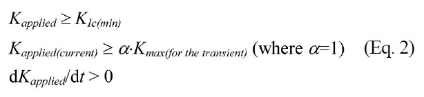
As noted in Eq. 1-2, FAVOR adopts a value
3.4.5.2 Crack Initiation Resistance Model
Our model includes the following five characteristics, all having functional forms motivated by an understanding of the physical processes responsible for cleavage fracture and numerical coefficients fit to empirical data:
A model of cleavage crack initiation fracture toughness that features a temperature dependence and scatter that is universal to all ferritic steels and is uninfluenced by irradiation, and a finite lower bound to the distribution of crack initiation toughness values (i.e., a value of fracture driving force below which cleavage fracture cannot occur). Our physical understanding of cleavage fracture suggests that the uncertainty (scatter) in fracture toughness should be modeled as aleatory. Because of this, in any individual probabilistic realization, FAVOR represents KIc as a distribution, not as a single value sampled from a distribution.
A model to account for the implicit conservatism in RTNDT: Our model recognizes that RTNDT is a conservative approximation to the true fracture toughness transition temperature, and so removes this conservative bias (on average). This bias is modeled as an epistemic uncertainty.
An irradiation damage model that recognizes that the effects of irradiation are purely athermal (i.e., affecting only the position of the fracture toughness transition curve on the temperature axis). This model, is a physically motivated fit to data from the United States Light Water Reactor (USLWR) surveillance program.
A model to convert between Charpy shift and fracture toughness shift due to irradiation: Recognizing that the shift in fracture toughness is not necessarily the same as the shift in Charpy V-notch energy quantified by the irradiation damage model, FAVOR incorporates a linear conversion between Charpy and fracture toughness shift [36].
Consideration of systematic material property variations throughout the beltline region: The specific properties (composition, unirradiated fracture toughness) of each weld, plate, and forging in the beltline are modeled explicitly in FAVOR, along with uncertainties in these variables. This refinement greatly exceeds that of previous PTS studies, where the entire beltline was modeled as having the fracture toughness of the most limiting component. Epistemic uncertainties in the properties of each beltline region are accounted for and propagated through the FAVOR calculation.
3.4.6 Through-Wall Cracking Model
Provided that
The crack arrest toughness model features a temperature dependence and an aleatory scatter of crack arrest toughness universal to all ferritic steels and not influenced by irradiation. Additionally, the crack arrest transition index temperature is related to the index temperature of the crack initiation toughness transition curve.
The upper shelf ductile initiation and tearing model features a temperature dependence and an aleatory scatter of upper shelf toughness universal to all ferritic steels and not influenced by irradiation. Additionally, there is a systematic relationship between the temperature at which the cleavage and ductile crack initiation toughness curves cross and index temperature of the crack initiation toughness transition curve [37].
3.5 Uncertainty Treatment and Propagation
Our approach considers a broad range of factors that influence the likelihood of vessel failure during a PTS event, while accounting for uncertainties in these factors across a breadth of technical disciplines [38]. Two central features of this approach are a focus on the use of realistic input values and models (wherever possible), and explicit treatment of uncertainties (using currently available uncertainty analysis tools and techniques). Thus, our current approach improves upon that employed in developing SECY-82-465, in which many aspects of the analysis included intentional and un-quantified conservatisms, and uncertainties were treated implicitly by incorporating them into the models (RTNDT, for example).
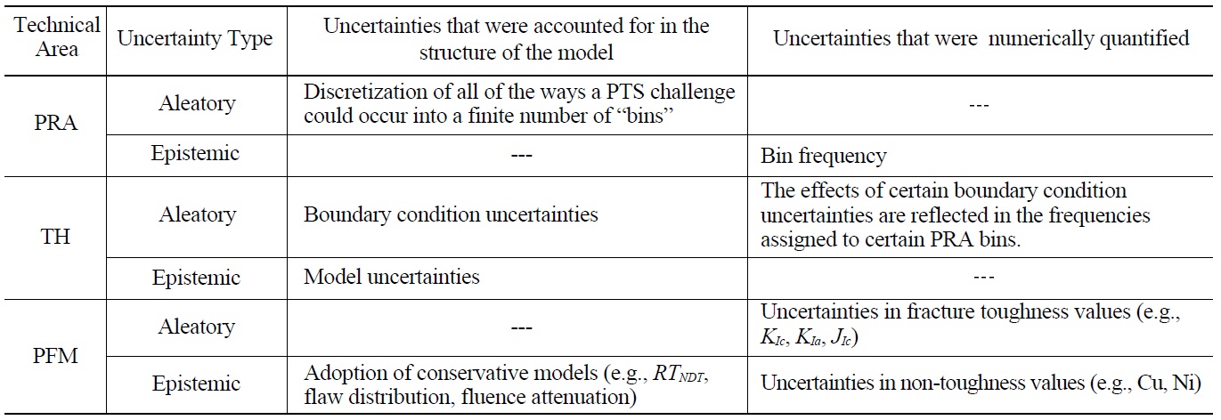
Our probabilistic models distinguish between aleatory and epistemic uncertainties. Aleatory uncertainties arise as a result of the randomness inherent in a physical or human process, whereas epistemic uncertainties are caused by limitations in our current state of knowledge (or understanding) of a given process. A practical way to distinguish between aleatory and epistemic uncertainties is that the latter can, in principle, be reduced by an increased state of knowledge. Conversely, because aleatory uncertainties arise as a result of randomness at a level below which a particular process is modeled, they are fundamentally irreducible. The distinction between aleatory and epistemic uncertainties is an important part of PTS analysis because different mathematical and/or modeling procedures are used to represent these different types of uncertainty.
While uncertainties in all parts of the PTS model have been systematically examined, not all have been numerically quantified as part of the model. Nevertheless, these unquantified uncertaintinties have still been accounted for in the model structure (e.g., via conservative binning of transients, by adoption of conservative models, etc.). Table 3 summarizes the uncertainty treatment for the three major parts of the PTS model.
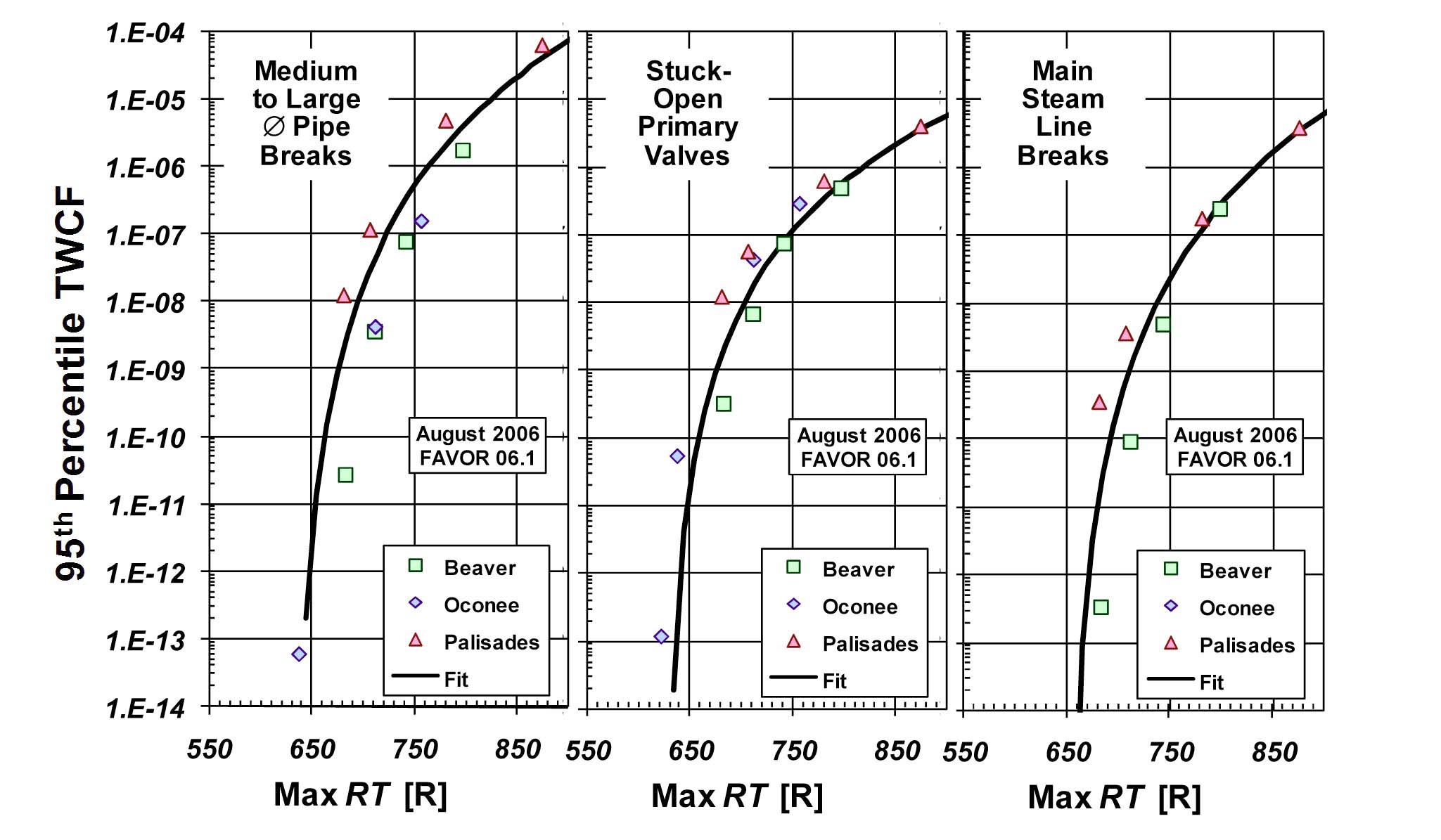
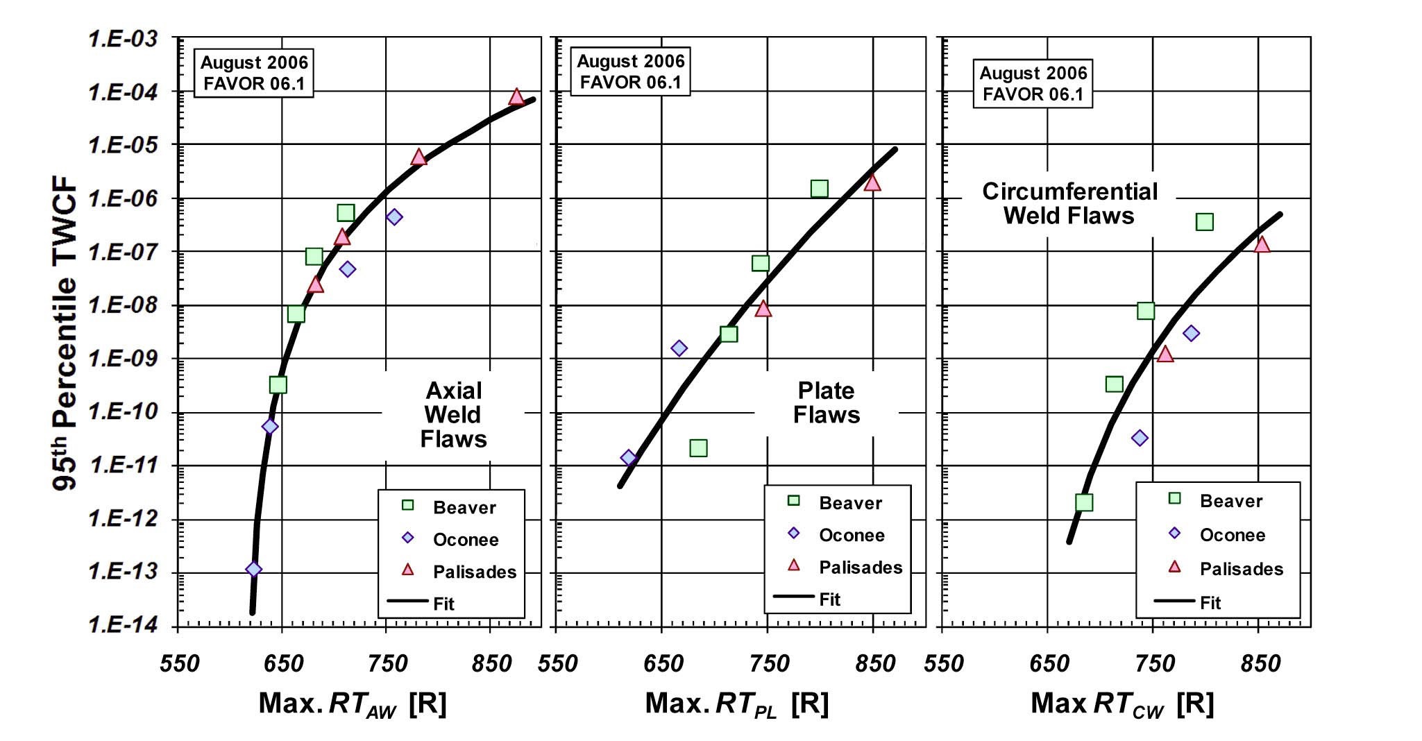
Fig. 4 and Fig. 5 summarize the key results from [4]. In Fig. 4 the 95th percentile of the TWCF distribution (TWCF95)† for different transient classes is plotted as a function of embrittlement, while Fig. 5 presents the variation of TWCF95 for different flaw populations with embrittlement. The following variables were used to quantify embrittlement; they appear on the abscissas of Fig. 4 and Fig. 5:
RTMAX-AW characterizes the resistance of the RPV to fracture initiating from flaws found along the axial weld fusion lines. Because these flaws sample both the toughness properties of the weld and of the adjacent plate, the value of RTMAX-AW is the higher of the RT for the weld and the plate. The value of RTMAX-AW for the vessel is the highest RTMAX-AW of any individual axial weld fusion line.
RTMAX-PL characterizes the resistance of the RPV to fracture initiating from flaws in plates that are not associated with welds. The value of RTMAX-PL for the vessel is the highest RTMAX-PL of any individual plate
RTMAX-CW characterizes the resistance of the RPV to fracture initiating from flaws found along the circumferential weld fusion lines. Because these flaws sample both the toughness properties of the weld and of the adjacent plate (or forging), the value of RTMAX-CW is the higher of the RT for the weld and the plate (or forging). The value of RTMAX-CW for the vessel is the highest RTMAX-CW of any individual circumferential weld fusion line.
Implications of the results in Fig. 4 and Fig. 5 are discussed in the following two sub-sections.
Our analysis assessed the contribution of a wide variety of transient classes to PTS risk, including primary-side pipe breaks, stuck-open valves on the primary side, main steamline breaks, stuck-open valves on the secondary side,
[Table 3.] Summary of Uncertainty Treatment in the Three Major Technical Areas
Summary of Uncertainty Treatment in the Three Major Technical Areas
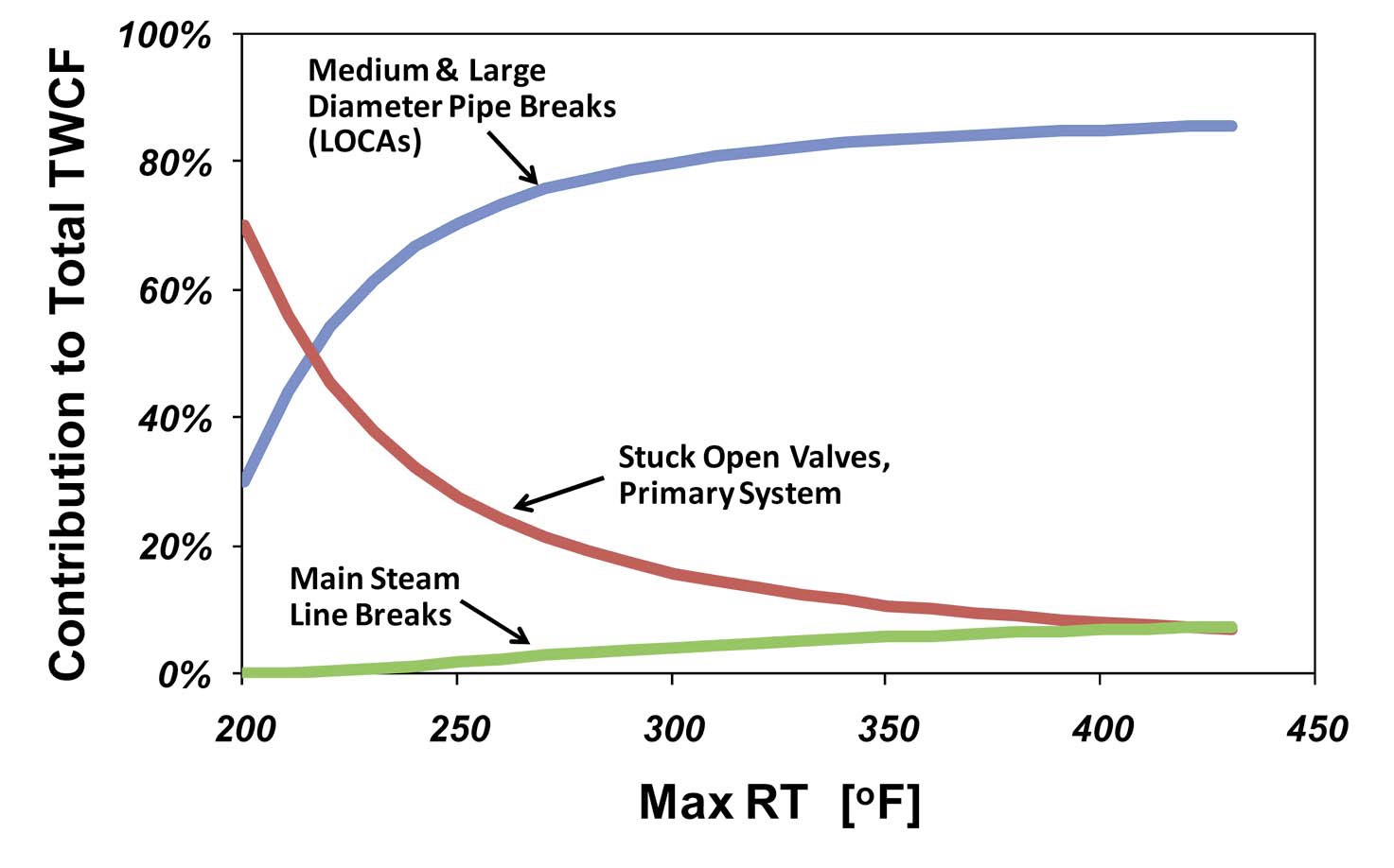
feed-and-bleed, steam generator tube rupture, and mixed primary and secondary initiators. Only the most severe transients make any significant contribution to the total TWCF. Fig. 4 shows the dependence on embrittlement of the TWCF95 caused by the dominant transient classes, while Fig. 6 shows the percentage of the total TWCF contributed by each transient class (transients not represented in these figures contribute less than 0.1% to the TWCF). The following paragraphs explore why some transients contribute to TWCF while others do not.
The most significant transient class is faults on the primary side, which collectively are responsible for 90% or more of the total TWCF. These faults fall into two subcategories: stuck open valves that may later re-close, and medium- to large-diameter pipe breaks. At low embrittlement levels (RTMAX-AW<?220 ℉) stuck open valves that may later re-close dominate the TWCF. While the initial cooling rate of these transients is modest, they cool the primary system to temperatures on the order of the injection water (50℉). At this low temperature re-pressurization may occur if operators do not realize that the valve has re-closed and throttle injection. Even though the fracture toughness is relatively high at these lower embrittlement levels, the stresses generated by re-pressurization can fail the vessel. At higher embrittlement levels medium- to largediameter pipe breaks dominate the TWCF. The rapid cooling rates and low downcomer temperatures generated by rapid depressurization and emergency injection of low-temperature makeup water combine to produce a high-severity transient.
Breaks of the main steam line (MSLB) are a small (< 10%) contributor. While MSLBs rapidly cool the inventory of the primary pressure circuit, they do not produce low temperatures in the primary system, which is limited to the boiling point of water in the secondary system. At this temperature, the RPV steel is sufficiently tough to resist failure most of the time.
Together these three transient classes make up nearly all of the TWCF; they exhibit remarkably little plant-to-plant variation in the US PWR fleet for the following reasons:
Stuck-open valves that may later re-close: When these transients cause failure they do so at the time of repressurization when the primary coolant temperature is invariably at, or near, that of the injection water. At re-pressurization the pressure goes to the safety valve
setpoint. These factors are similar across the operating fleet in the United States. While operator actions influence the characteristics of these transients early on, at the time failure is predicted the effect of operator action is negligible
Medium to large diameter pipe breaks: Once the size of the pipe break exceeds 6- to 8-in. in diameter the temperature of the primary coolant water is falling so rapidly that the temperature of the steel in the RPV wall cannot keep up due to its finite thermal conductivity. The cooling rate of the vessel wall, and thus the thermal stress, is therefore controlled by two factors: the thermal conductivity of the steel, and the thickness of the vessel wall. The similarity of PWR diameters in the US fleet leads to a roughly equivalent challenge being posed to all RPVs by this transient class. Operator action is not a factor as the only possible operator action is to maximize the injection of water so as to keep the core covered.
Main Steam Line Breaks: If a RPV failure is predicted as a result of a MSLB it will be predicted very early in the transient, long before any operator action could credibly occur. At these times the transient characteristics are dominated by the extremely fast initial cooling rates, which are similar across the RPV fleet due to the fact that the cooling rate of the RPV inventory is far faster than can be achieved in the wall of the RPV, so plant-specific differences in steam-line diameter cannot influence the TWCF.
4.2 Dominant Material Features
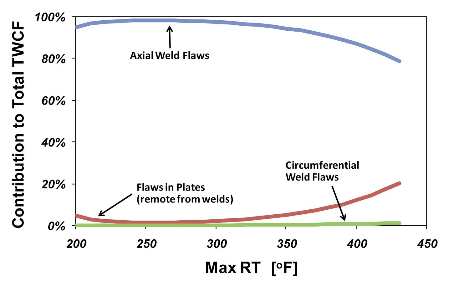
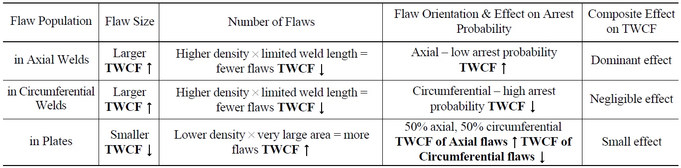
Fig. 5 shows the relationship between three RT metrics, RTMAX-AW, RTMAX-PL, and RTMAX-CW, and the TWCF95 resulting from three flaw populations: axial fusion line flaws in axial welds, axial and circumferential flaws in plates, and circumferential flaws in circumferential welds (respectively). Fig. 7 places all three curve-fits from Fig. 5 on a single graph, which makes clear that axial weld flaws dominate the TWCF. These significantly different TWCFs arising
from different flaw populations can be understood based on three factors that are all summarized in Table 4: flaw size, the number of flaws in the vessel, and flaw orientation. The relative effects of flaw size and orientation are easily understood (bigger flaws are worse, more flaws are worse); Table 4 details differences in flaw sizes and numbers for the different flaw populations modeled. The effect of flaw orientation (axial or circumferential) is critically important because of its effect on the likelihood of crack arrest. Cheverton et al. describe how the application of a cold thermal shock to the inner diameter of a cylinder containing a flaw produces bending of the cylinder wall [39]. This bending, originating from the contraction of the cold metal at and near the ID and the resistance to this contraction provided by the hotter metal at the OD, tends to be much larger for axial flaws (an asymmetric geometry) than for circumferential flaws (a symmetric geometry). The asymmetry associated with the axial flaw degrades the cylinder's resistance to bending, which produces an applied-
To assess the applicability of these findings to US PWRs in general, a number of “generalization studies” were performed. These studies revealed the following:
TH Sensitivity Studies: No credible effects were discovered that changed the results significantly enough to recommend changes to the baseline RELAP model, or to recommend cautions regarding the robustness of those models.
[Table 4.] Effect of Flaw Population on TWCF

Effect of Flaw Population on TWCF
PFM Sensitivity Studies: No credible effects were discovered that changed the results significantly enough to recommend changes to the baseline FAVOR model. However, these studies revealed that the baseline studies did not address the effects of vessel wall thickness adequately, nor did they provide the basis for establishing RT-limits for ring-forged vessels. Further work on both topics appears in Section 5.
Design and Operational Characteristics of other PWRs: With the exception of stuck-open valves at low levels of embrittlement a study of five additional PWRs revealed no differences in sequence progression, sequence frequency, or plant thermal-hydraulic response significant enough to call into question the applicability of the TWCF results from the three detailed plant analyses to PWRs in general. A minor inadequacy of the three detailed plant analyses to entirely treat stuck-open values was addressed by introduction of the α-factor (see Section 5).
External Events: An investigation of external initiating events (e.g., fires, earthquakes, floods) showed the contribution of those events to the total TWCF is negligible.
† Because of the skewness in the distribution of TWCF values, the mean of these distributions corresponds to a very high percentile value (above the 80th percentile for all embrittlement levels studied). TWCF95 was adopted to provide a consistent basis for comparison between all analyses.
5. USE OF THESE FINDINGS TO ESTABLISH REGULATORY LIMITS
The information presented in Section 4 demonstrates that the three study plants represent the population of PWRs operating in the USA well subject to the following restrictions:
The results for the study plants underestimate slightly the TWCF from stuck-open valves on the primary side that may later reclose at low embrittlement levels,
The results for the study plants do not capture the effect of RPV thickness on TWCF, and
The study plants do not represent the effects of forging flaws.
In view of these restrictions provisional regulatory limits were first developed based only on the results from the three study plants. These provisional limits were then modified, based on the results of sensitivity studies, to remove these restrictions. The remaining information in this section describes this process.
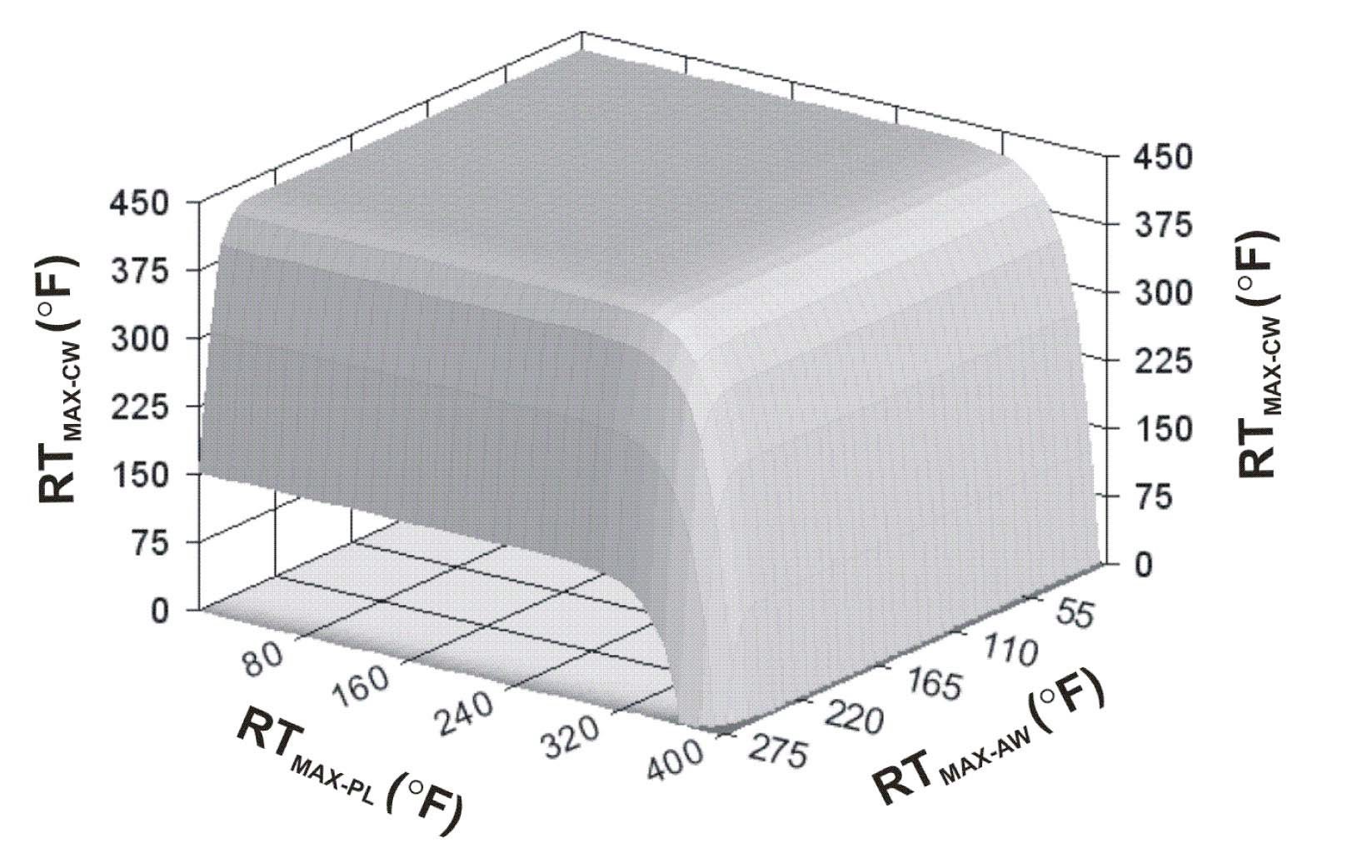
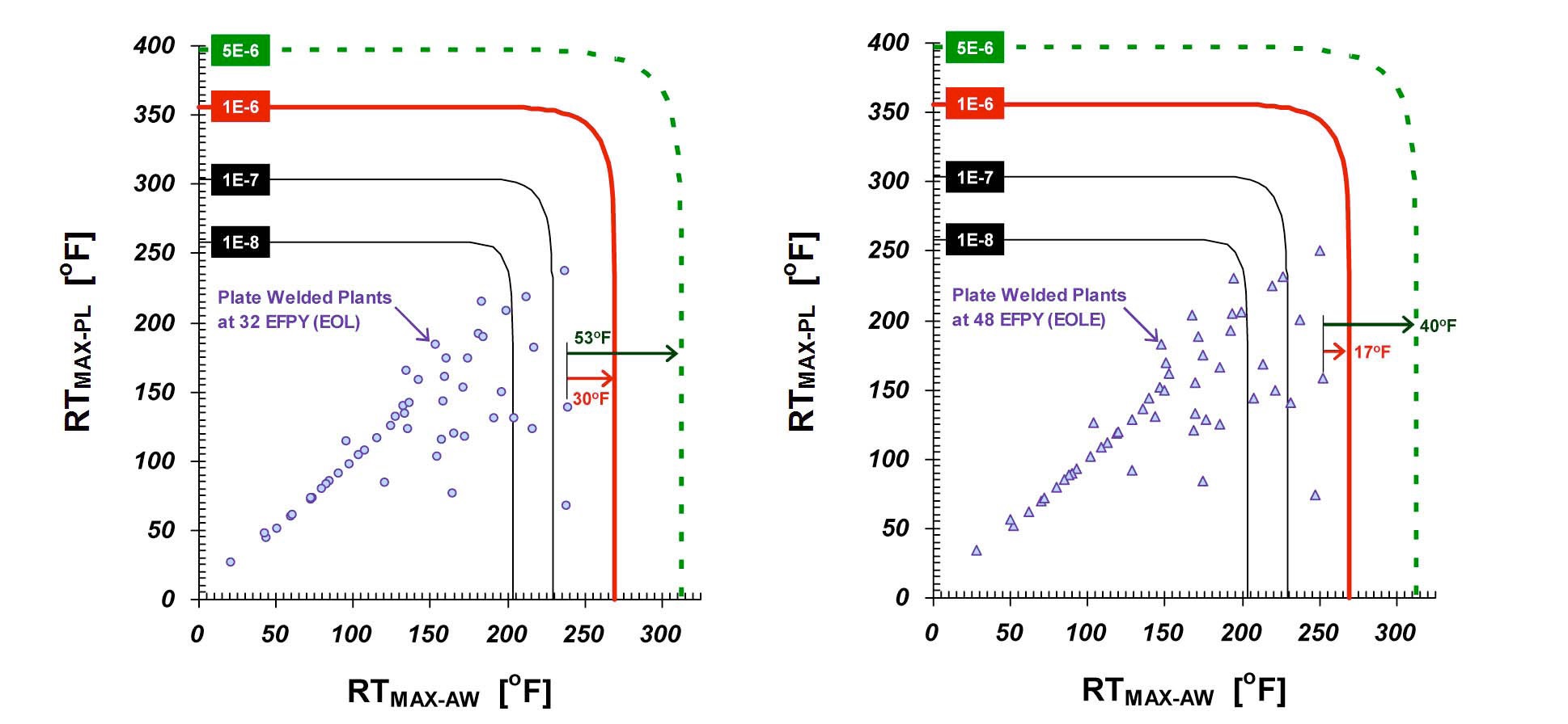
The fits to the TWCF95-xx versus RTMAX-xx relationships shown in Fig. 5 can be added together to develop a relationship that estimates the total TWCF95 that can be expected for a plate welded RPV based on the level of embrittlement experienced by its constituent parts. Fig. 8 provides a graphical depiction of this relationship. The 3D surface in the figure represents the combinations of RTMAX-AW, RTMAX-PL, and RTMAX-CW that produce a total TWCF95= 1x10⁻⁶/ry. This figure provides a tool by which operating plate welded RPVs can be assessed. By plotting the embrittlement characteristics of each RPV (as quantified by RTMAX-AW, RTMAX-PL, and RTMAX-CW) in the 3D space of Fig. 8 one can quickly determine if a particular RPV is predicted to have a TWCF95 below 1x10⁻⁶/ry (i.e. points plotting inside the surface) or above 1x10⁻⁶/ry (i.e. points plotting outside the surface). Fig. 9 provides such a plot for all currently operating plate-welded PWRs in the USA for purposes of illustration (in this plot, the negligible effects of circumferential
weld flaws have been ignored for clarity; this simplification permits representation of the 3D surface in Fig.8 in 2D).
As stated previously, the provisional limits shown in Fig. 5 require modification to address all conditions of interest for PWRs operating in the USA. These modifications, which are based on sensitivity studies described in [\40], are as follows:
Stuck Open Valves: When the results from the three study plants were compared to a larger population of RPVs in the generalization study it was determined that the TWCF produced by stuck open valves that may later re-close is under-estimated by up to a factor of 2.5 for plants that have a much smaller RCS volume than did the study plants. To address this deficiency a factor (α) was introduced in the derivation of the final limits. The α factor is a 2.5 multiplier at low embrittlement levels that diminishes to 1 at high embrittlement levels because, as shown in Fig. 6, the influence of stuck open valves on the total TWCF diminishes as embrittlement increases.
Vessel Wall Thickness: The wall thickness of all three study plants is 8 to 8½-in., which is characteristic of the vast majority of PWRs in the USA. However, three PWRs are thicker (11-11½-in.) while seven are thinner (6½-7-in.). The magnitude of the stresses produced by thermal shock increase with wall thickness because thicker vessels are stiffer. Sensitivity studies performed to investigate this effect found that, with all other factors held constant, the TWCF could increase by between 8x and 40x (depending on the transient) as vessel wall thickness is increases between 8 and 11 inches. To address this deficiency a factor (β) was introduced in the derivation of the final limits. The β multiplier increases the TWCF by a factor of 8 for each inch of thickness by which the vessel exceeds 9½-in. (TWCF is not reduced for thinner vessels, which is conservative).
Forging Flaws, Embedded: Forgings have a population of embedded flaws that is particular in density and size to their method of manufacture. The sensitivity studies in [4] revealed that embedded flaws in forgings are similar in both size and density to the embedded flaws in plates modeled in the three study plants. Consequently the relationship between RTMAX-PL and TWCF95 (see center graph, Fig. 5) was adopted to characterize embedded flaws in forgings.
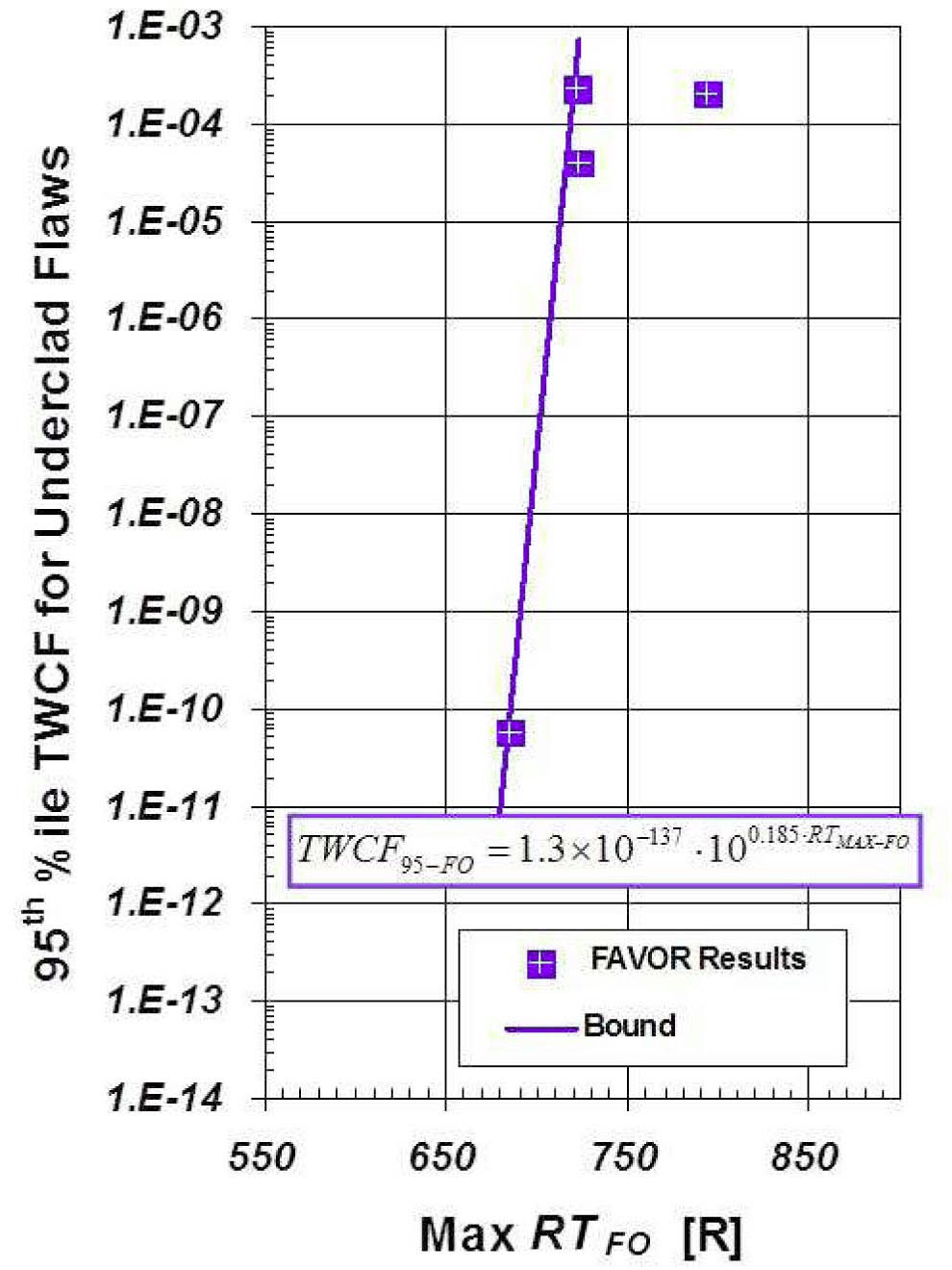
Underclad Cracks in Forgings: Forgings may contain underclad cracks that are produced by the deposition of the austenitic stainless steel cladding layer. Underclad cracks occur as dense arrays of shallow cracks extending into the vessel wall from the clad-to-base metal interface to depths that are limited by the extent of the heataffected zone. These cracks are oriented normal to the direction of welding for clad deposition, producing axially oriented cracks in the vessel beltline. Available information from the literature was used to establish a flaw distribution for underclad cracks, which was used as input to FAVOR. Fig. 10 summarizes the results of these analyses. The rate of increase of TWCF with increasing embrittlement for underclad cracks is much more rapid than shown previously (see Fig. 4) for plate and weld flaws. The steepness of this slope occurs because of the very high density of underclad cracks assumed in the analysis (the mean crack-to-crack spacing is on the order of millimeters), which means it is a virtual certainty that an underclad crack will occur in locations of high embrittlement. The data in Fig. 10 was used, together with that from Fig. 5, to establish the final PTS screening limits for forgings.
Collectively, the information presented in the preceding paragraphs provides the basis to augment the provisional procedure expressed in Fig. 8 and Fig. 9, thereby enabling the development of a general equation that can be used to estimate the TWCF95 for any operating PWR in the USA based only on input information regarding material embrittlement.
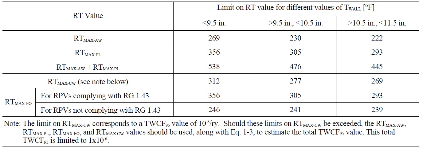
[Table 5.] RT Limits for PWRs to Ensure that TWCF95 Remains Below 10-6/ry

RT Limits for PWRs to Ensure that TWCF95 Remains Below 10-6/ry
This procedure can be expressed in two equivalent ways: either in terms of a limit placed on TWCF (see Eq. 1-3), or in terms of a limit placed on the various reference temperature (RT) metrics (see Table 5).
where
and the factors
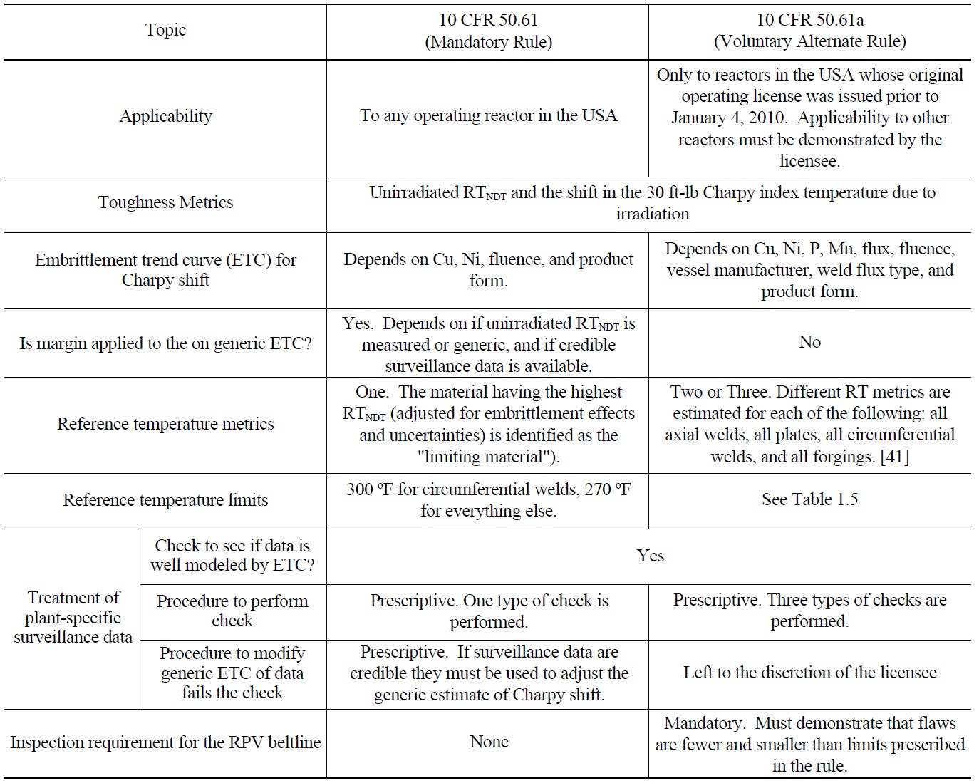
[Table 6.] Comparison of the Requirements and Procedures of 10 CFR 50.61 and 10 CFR 50.61a.

Comparison of the Requirements and Procedures of 10 CFR 50.61 and 10 CFR 50.61a.
6. RULES FOR ASSESSMENT OF PLANTS RELATIVE TO REGULATORY LIMITS
As of the publication date of this document, the following two rules in the United States Code of Federal Regulations (CFR) pertain to PTS:
10 CFR 50.61: The mandatory rule [2]
10 CFR 50.61a: The voluntary alternate rule [7]
The mandatory rule has been in force since 1984, its technical basis is detailed in [1]. The technical basis for the voluntary alternative rule was summarized in this Paper and is described in detail in [3,4,26,40]. Table 6 compares the provisions of the two rules. A major difference is that the RT-limits of the alternate rule are more detailed, and permit higher embrittlement levels to occur. These higher permitted embrittlement levels are justified by the increased accuracy of the modeling, data, and physical understanding that provides the technical basis for the alternative rule. However, a significant entry condition must be met to use the alternate rule: a vessel inspection must be performed so that the flaws that may exist in the vessel may be compared to the flaws that were assumed in the derivation of the RTlimits of the voluntary alternative rule.


![TWCF Fractions for the Three Study Plants Attributable to Different Broad Classes of Transients [4].](http://oak.go.kr/repository/journal/12381/OJRHBJ_2013_v45n3_277_f004.jpg)
![TWCF Fractions for the Three Study Plants Attributable to Different Flaw Populations [4].](http://oak.go.kr/repository/journal/12381/OJRHBJ_2013_v45n3_277_f005.jpg)

![Graphical Representation of the Curve Fits in Fig. 6. The TWCF of the Surface shown is 1x10⁻⁶, so Inside the Surface (Toward the Origin) the TWCF Less, while Outside the Surface the TWCF Exceeds 1x10⁻⁶ [4].](http://oak.go.kr/repository/journal/12381/OJRHBJ_2013_v45n3_277_f008.jpg)
![Maximum RT-based Screening Criterion (1E-6 Curve) for Plate-welded Vessels (Left: Screening Criterion Relative to Currently Operating PWRs after 40 years of Operation; Right: Screening Criterion Relative to Currently Operating PWRs after 60 years of Operation [4].](http://oak.go.kr/repository/journal/12381/OJRHBJ_2013_v45n3_277_f009.jpg)
![Relationship between TWCF and RT for Forgings Having Underclad Flaws [4]](http://oak.go.kr/repository/journal/12381/OJRHBJ_2013_v45n3_277_f010.jpg)