The IAEA (International Atomic Energy Agency) is coordinating a research project (CRP) named “Benchmark Analysis of Sodium Natural Convection in the Upper Plenum of the MONJU Reactor Vessel.” The CRP aims to validate the present multi-dimensional computational fluid dynamics (CFD) and turbulence models for predicting the thermal stratification in the upper plenum of a fast reactor. The JAEA sponsors this CRP and has provided a detailed geometrical data and time-dependent inlet conditions of the flow rate and temperature for the transient analysis. KAERI is a participant of the CRP with the other participants being ANL (USA), CEA (France), IPPE (Russia), IGCAR (India), CIAE (China) and JAEA (Japan). All the participating institutes were asked to perform calculations for the same problem, but with different numerical methods or turbulence models. The present work was done as a participant of this IAEA CRP.
An understanding of the thermal hydraulics in the upper plenum of a fast nuclear reactor is very important for securing reactor safety and the structural integrity of a solid structure. If the reactor is scrammed, the power of the reactor decreases rapidly and the coolant flow rate is reduced. Since the rate of power decrease is faster than the decrease of the flow rate of the coolant, the temperature of the coolant from the reactor core drops quickly over time. The cold coolant from the reactor core enters the lower region of the hot pool slowly owing to a density difference, and a large portion of the coolant in the upper plenum remains hot. This phenomenon invokes a thermally stratified condition and leads to a stiff axial temperature gradient in the vessel and upper internal structures. The stiff temperature gradient may cause severe thermal stress which may deteriorate the structural integrity of the components in the upper plenum.
Several experimental and numerical works [1-5] have been done in the past to understand and provide a computational tool to analyze the thermal stratification phenomenon. A large-scale sodium experiment to investigate the thermal stratification phenomenon is expensive and difficult, owing to the opaque nature of sodium and the possible chemical reaction with air or water. However, a thermal sodium experiment cannot be replaced by a water or air experiment, owing to a large difference in the Prandtl number. Thus, the CFD approach can be a valuable tool to investigate the thermal stratification in the upper plenum of a sodium-cooled fast reactor. However, the CFD approach is not free from difficulties in the prediction of thermal stratification, and the accuracy of the numerical solution is greatly dependent on the turbulence model used and the treatment of the convection terms. Most of the turbulence models have been developed mainly for forced convection flows, and more advanced turbulence models for buoyancy dominated flows are not yet available in commercial CFD codes such as FLUENT, CFX, and STAR-CD, although they are well established in the literature, including works by Hanjalic [6] and Choi and Kim [7].
The earlier numerical work by Muramatsu and Ninokata [4] showed that the choice of the turbulence model and the treatment of the convection scheme are important for a proper prediction of the thermal stratification. They showed that the use of an algebraic stress and flux turbulence model and a higher-order convection scheme are efficient for analyzing the thermal stratification. The treatment of higher-order convection term is well implemented in commercial codes. However, the treatment of the Reynolds stresses and turbulent heat fluxes requires special attention since the accuracy of the numerical solution is highly dependent on the turbulence model used, especially in the analysis of natural convection flows with thermal stratification.
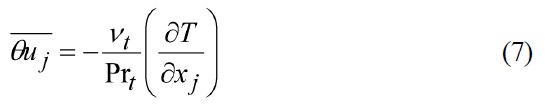
One of the difficulties in predicting turbulent natural convection is the treatment of turbulent heat fluxes. If one does not use a differential heat flux model, a proper way of treating the turbulent heat fluxes should be sought. Most commercial codes employ a simple gradient diffusion hypothesis (SGDH) in treating the turbulent heat fluxes, which is expressed in Eq. (7). The SGDH works well for forced convection flows; however, it does not produce accurate solutions for natural convection flows. Ince and Launder [8] proposed a generalized gradient diffusion hypothesis (GGDH) to overcome this deficiency of the SGDH. The GGDH works very well for shear dominant flows; however it produces unstable and inaccurate solutions for strongly stratified natural convection flows. To remedy this deficiency, Hanjalic [6] proposed an algebraic flux model (AFM). The main difference between the AFM and GGDH is the inclusion of a temperature variance term in the algebraic expression of the turbulent heat fluxes. This inclusion of the temperature variance term stabilizes the overall solution process and results in a stable and accurate solution. However, the AFM requires one more numerical solution of a partial differential equation for the temperature variance than the GGDH. A detailed analysis on the treatment of a turbulent heat flux for the computation of turbulent natural convection flows is given in Choi and Kim [9]. Since the GGDH and AFM are not implemented in the CFX-13 code, the calculations were performed using the SGDH in the present study. The computation of thermal stratification using the SGDH usually causes an over-prediction of the turbulent heat fluxes and expedites the thermal mixing as shown in Pellegrini et al. [10].
As for treatment of the Reynolds stresses, more advanced turbulence models have been developed during the last two decades, and the turbulence models commonly used at present are the two-layer
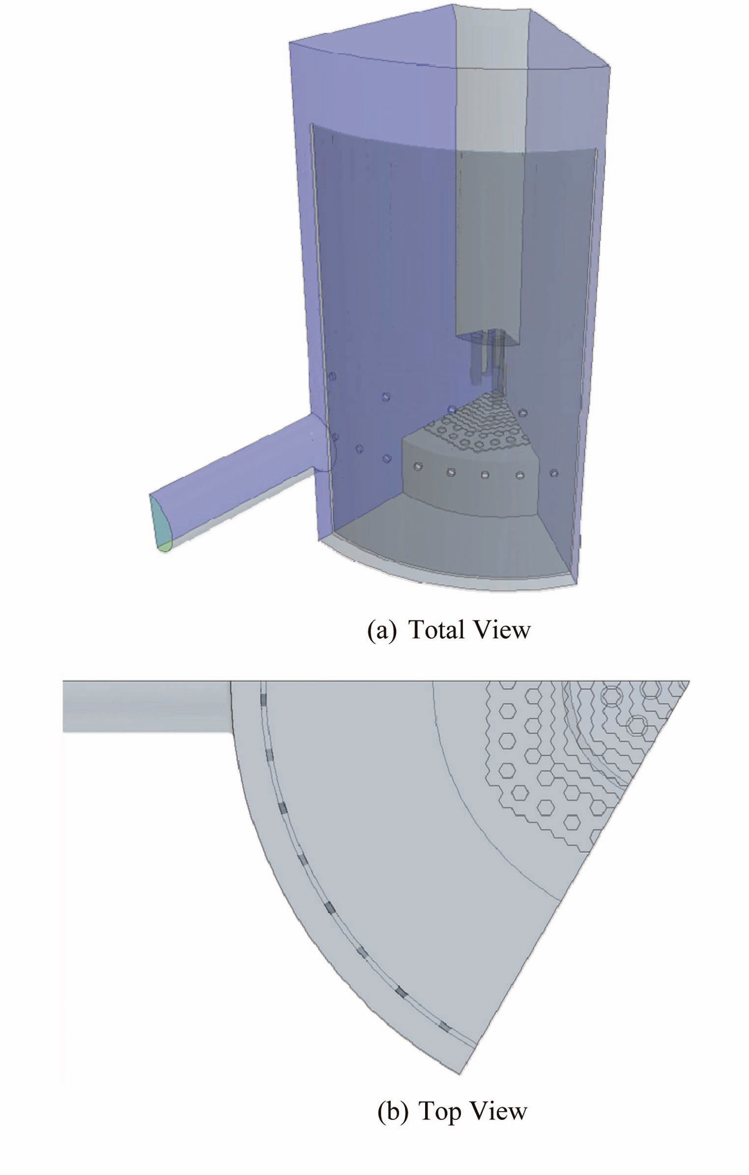
In addition to the turbulence modeling problem, another numerical issue for the computation of the fluid flow and heat transfer in the upper plenum of the MONJU fast reactor is the treatment of the geometrically complex upper core structure and other structures in the upper plenum shown in Figs.1-2. In the present study, a porous media approach is employed to handle the complicated geometry efficiently, and the detailed treatment of the porous media approach will be given in section 4.5. To reduce the vast computer storage required in the present simulation, a simplified 1/6 symmetric model of the upper plenum is employed for computation.
In the following sections, a brief explanation of the upper plenum of the MONJU reactor and a mathematical formulation of the governing equations and turbulence model are given, followed by an explanation of the numerical method, the results and discussion, and finally, some concluding remarks.
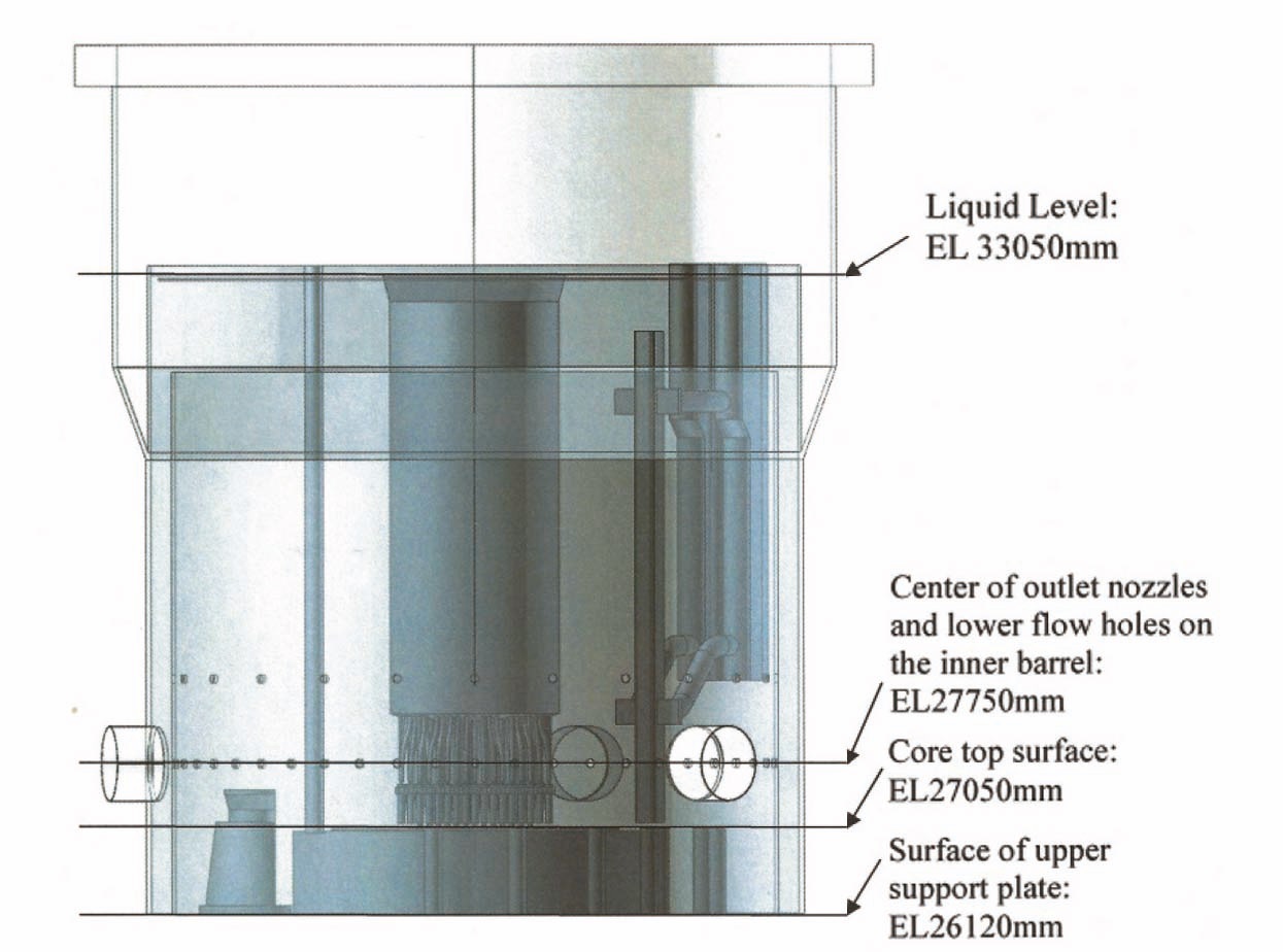
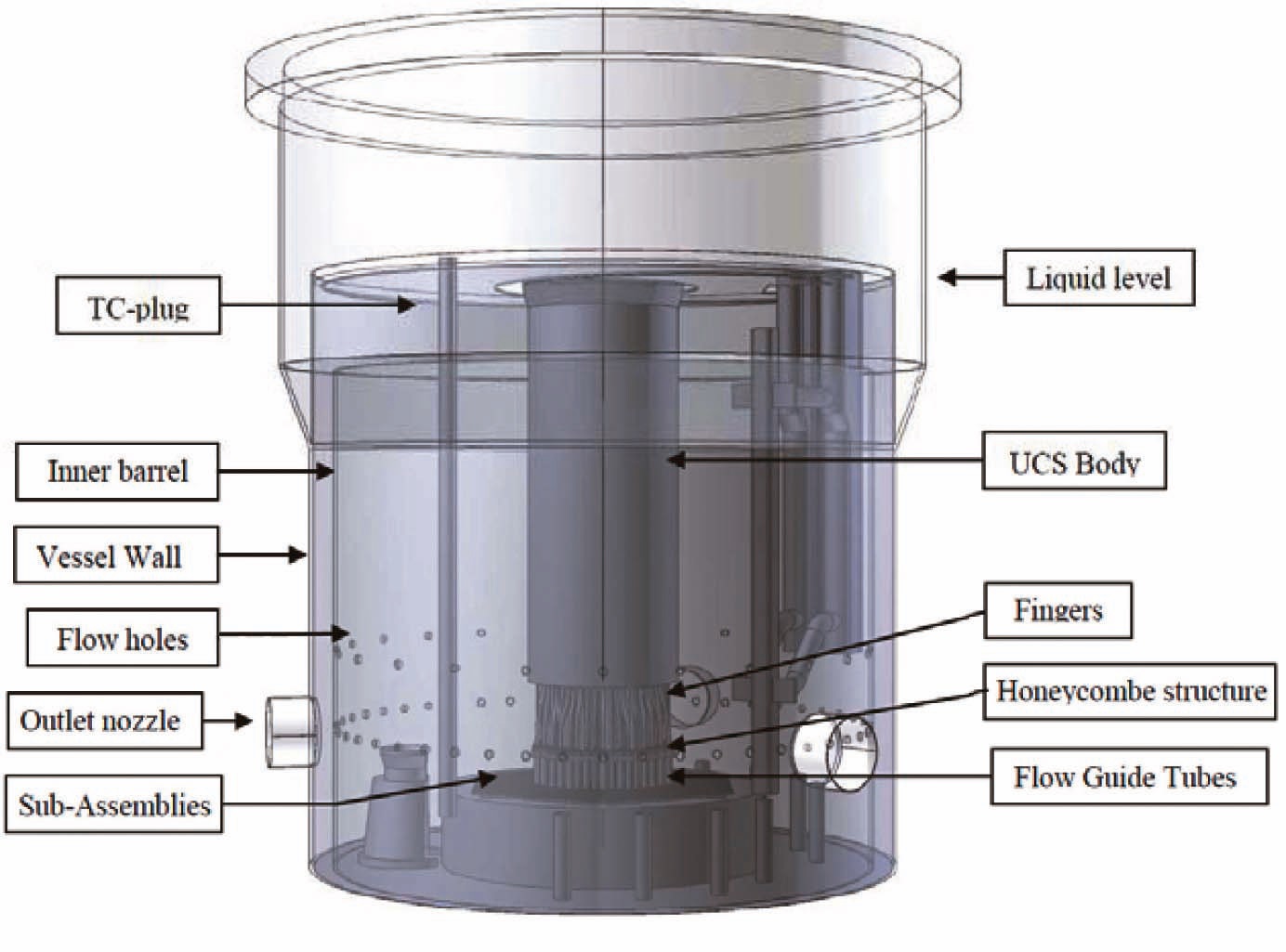
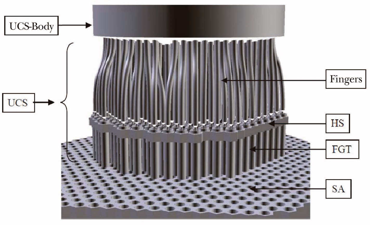
The MONJU reactor is a 714MWt (280MWe) loop type (3 loop) sodium cooled fast reactor located near Tsuruga, Japan. The core of the MONJU reactor consists of conventional driver fuel assemblies with two enrichment zones, blanket fuel assemblies, neutron shields and control rods. A complete view of the upper plenum of the MONJU reactor is shown in Fig. 1-(a) and the elevation levels of important positions inside the reactor upper plenum is shown in Fig. 1-(b). These figures and the experimental data are provided by JAEA [15]-[16]. The reactor vessel is a vertical cylindrical vessel with three outlet nozzles. There are two rows of flow holes in the inner barrel which is located inside the reactor vessel. The upper core structure (UCS) is situated above the sub-assembly outlets and below the UCS-body, as shown in Fig. 2. The UCS consists of a honeycomb structure (HS), flow-guide tubes (FGT),
and fingers. The thermocouples used to measure the fuel assembly outlet temperature are located inside the fingers. The 19 control rod guide tubes are present inside the UCS. The 36 thermocouples are located at the thermocouple plug to measure the vertical temperature distribution during the turbine trip test. The sodium flows out of the subassembly, passes inside the flow guide tube to enter the fingers region vertically, and moves into the upper plenum. The sodium flow then passes through either the flow holes in the inner barrel or passes above the inner barrel, before finally flowing out of the vessel at the outlet nozzle. Since thermal stratification was limited to the upper plenum, only the portion of the reactor vessel above the core support plate is considered in the present analysis.
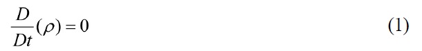
The ensemble-averaged governing equations for the conservation of mass, momentum, and energy can be written as follows;
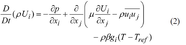
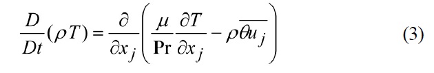
where

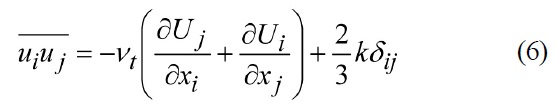
are the Reynolds stresses and

are the turbulent heat fluxes which should be modeled.
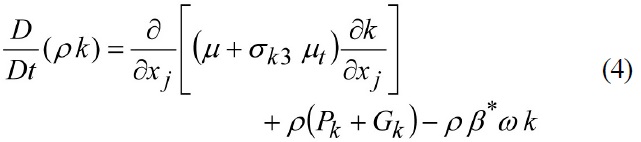
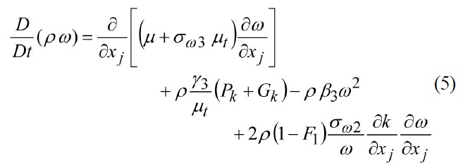
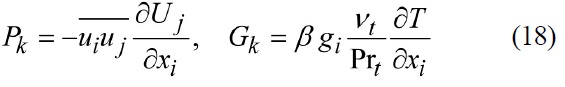
The turbulence model employed in the present simulation is the shear stress transport (SST) model by Menter [12]. In this model, the transport equations for the turbulence kinetic energy (k) and its frequency (ω) are solved. The governing equations for k and ω are as follows;
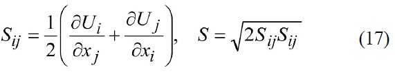
In this model the Reynolds stresses and turbulent heat fluxes are expressed as follows;
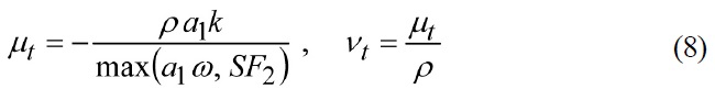
where the turbulent eddy viscosity is given as follows;

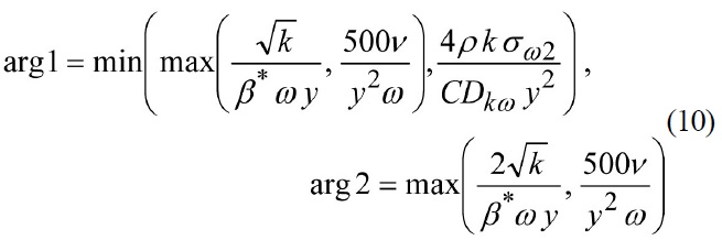
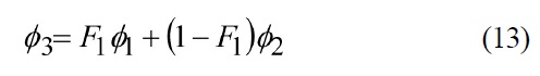
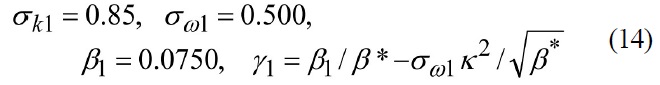
The coefficients of the SST model are a linear combination of the corresponding coefficients such that
where
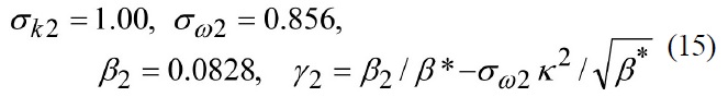
and
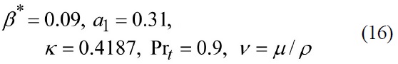
The time-dependent mass flow rate and temperature are prescribed at the each subassembly outlet using the experimental data provided by JAEA [16]. The mass flow rate and temperature at each subassembly are assumed to be spatially uniform. The turbulent kinetic energy and its frequency are specified using the turbulence intensity (5%) and the geometric data of each subassembly outlet. All the walls are treated as adiabatic, and no slip boundary condition is specified at the wall since the calculation is carried out all the way to the wall without using the wall functions. The symmetry condition is specified at the two lateral surfaces of the 60° geometry. The pressure boundary condition is specified at the outlet nozzle.
4.1 The Simplified Geometric Model
Sofu et al. [17] developed a simplified CAD model and distributed it to all CRP participants. In this model only 1/6 of the upper plenum of the MONJU reactor is considered. A 60° section is modeled, where the following modifications have been made to obtain a symmetric geometry.
- All of the subassembly outlets are taken as hexagonal;
- The top of the subassembly outlets are placed on different levels to distinguish the different channels easily;
- The outlet nozzle is rotated with respect to the hexagonal core configuration (only half of the outlet nozzle is modeled);
- The internal structures of the upper plenum like ‘invessel transport machine’, ‘low guide’, or ‘thermocouple plug’ are not modeled.
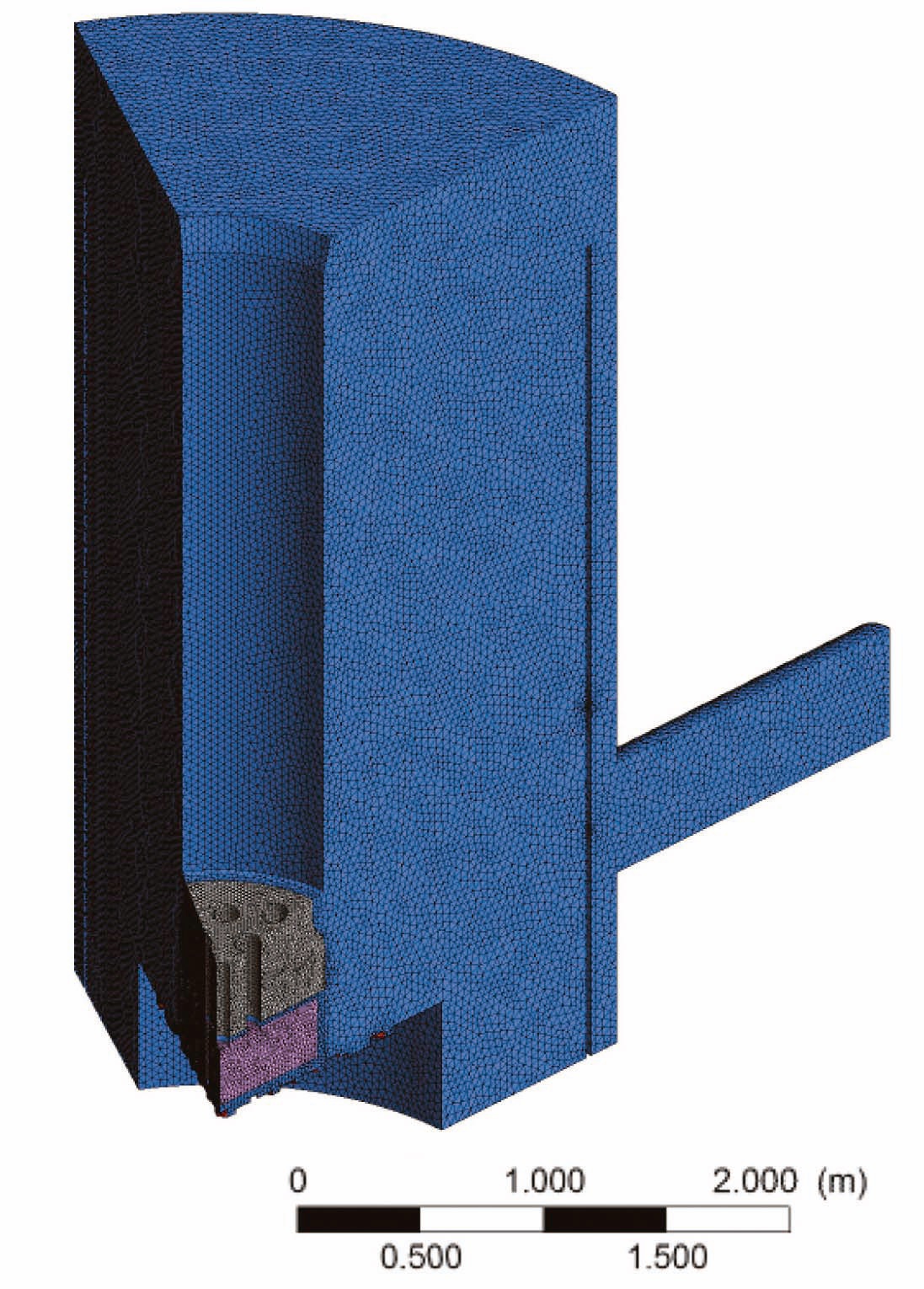
Within the upper core structure, only the control rod guide tubes are realized in the CAD model. The flow guide tubes and thermocouple fingers are not treated explicitly owing to their small size and geometrical complexity. Fig. 3 shows the symmetric 1/6 simplified model developed by Sofu et al. [17].
Using the CAD model of the simplified 60° geometry, the numerical grids are generated with the ICEM CFD software. A total of 1.3 million tetrahedral elements are generated in the whole computational domain Fig. 4 shows the numerical grids employed in the present study for a simulation of the whole solution domain.
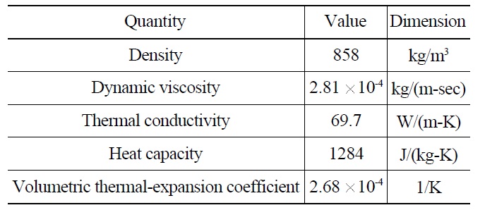
Liquid sodium is used as a coolant in the MONJU reactor. The physical properties are assumed to be constant for the whole computational domain, which means that the physical properties do not vary with temperature. The reference temperature is 400℃, and the physical properties of sodium at this reference temperature are given in Table 1.
Computations are carried out using the commercial code CFX-13 and the details of the numerical scheme are summarized in Table 2.
Blind et al. [18] proposed the following porous media approach for the UCS of MONJU reactor and it is also used in the present study. The pressure loss at the upper core structures and the associated porous media formulation are analyzed. The flow guide tubes and fingers in the upper
[Table 1.] Physical Properties of Sodium at 400℃

Physical Properties of Sodium at 400℃
[Table 2.] Summary of Numerical Scheme
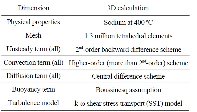
Summary of Numerical Scheme
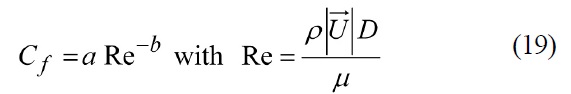
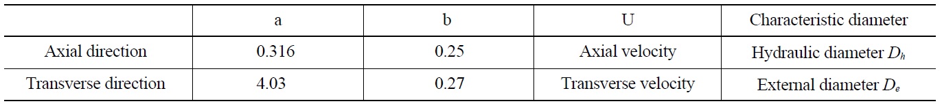
core structure are filled with tube bundles, and the pressure loss coefficient in these regions is expressed in the following form;
The associated frictional force is given by
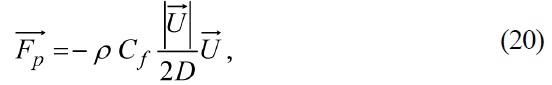
where D is the characteristic diameter. Table 3 shows the values of constants for the present porous media model. In the present analysis, the volumetric porosity in the fingers region is specified as 0.83. The hydraulic diameter (
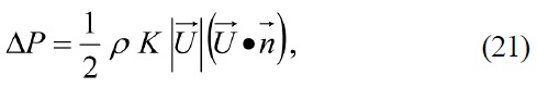
where the value of pressure loss coefficient K is equal to 60.
A steady-state computation is performed to provide the initial condition for a transient simulation. The usual steady-state calculation method does not work well for a convergence of the temperature field. The time marching strategy with a time step size of Δ
[Table 3.] Parameters for the Pressure Loss Correlation
Parameters for the Pressure Loss Correlation
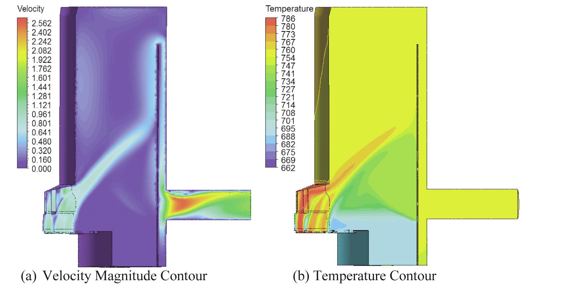
a complete convergence after 70,000 time marching. Fig. 5 (a)-(b) shows the steady-state velocity magnitude and temperature contour plots on the symmetry plane through the outlet. The hot sodium from the core spreads conically outward and then moves upward along the inner surface of the inner barrel. Owing to this strong flow, there exists a relatively weak counter current along the vertical surface of the upper structure main body, resulting in a large toroidal recirculation zone above the core outlet level. The sodium in the annular region between the inner barrel and reactor vessel flows downward and flows out of the reactor at the outlet. Below the core outlet level, the flow field is almost stagnant with significantly colder sodium. It is noted that the sodium in most of the upper plenum and outlet region is well mixed and the temperature of the sodium is nearly uniform. Small flow holes on the inner barrel do not play a significant role in mixing the fluid on the opposing sides of the inner barrel for the steady-state conditions.
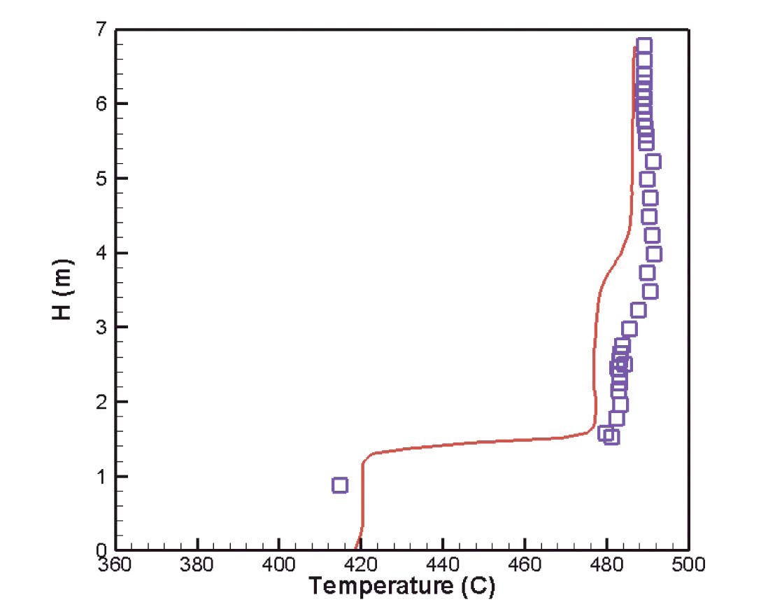
Fig. 6 shows the predicted vertical temperature distribution along the thermocouple tree (shown as TC plug in Fig.1-(a)) together with the experimental data. The predicted temperature distribution agrees fairly well with the experimental data, especially when the complex structures of the core upper plenum and the assumptions introduced for the 1/6 simplified model are considered. It was noted that the temperature varies rapidly at a height of y=1.4 m, and does not vary significantly above this height, which is consistent with the temperature distribution shown in Fig. 5-(b).
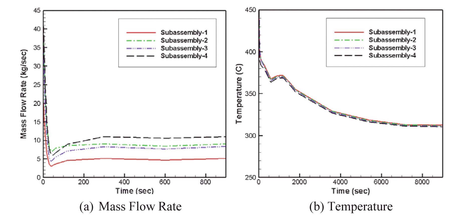
The transient computation is performed using the steady-state solution as an initial condition. The size of the time step should vary with the flow variation after the primary pump trip. The general features of the coastdown of the mass flow rate and temperature of the subassemblies near the core center are shown in Fig. 7. The data in Fig. 7 are provided by JAEA [16]. The notation “subassembly- 1” in Fig. 7 means the channel-1 of the core-1 in the MONJU reactor [16]. This figure shows that the mass flow rate drops very rapidly down to about 20% of the initial, steady-state value within one minute after the primary pump trip. The flow rate then increases slowly until 300 seconds, and remains nearly constant after 300 seconds. It was noted that the coastdown behavior of the temperature field is a little different from that of the mass flow rate. The temperature drops rather slowly compared to the mass flow rate until about 500 seconds, then increases slightly, and drops gradually until about 8000 seconds.
The size of the time step is chosen following the above coastdown behaviors of the mass flow rate and temperature. In the first minute of the simulation, a time step size of Δ
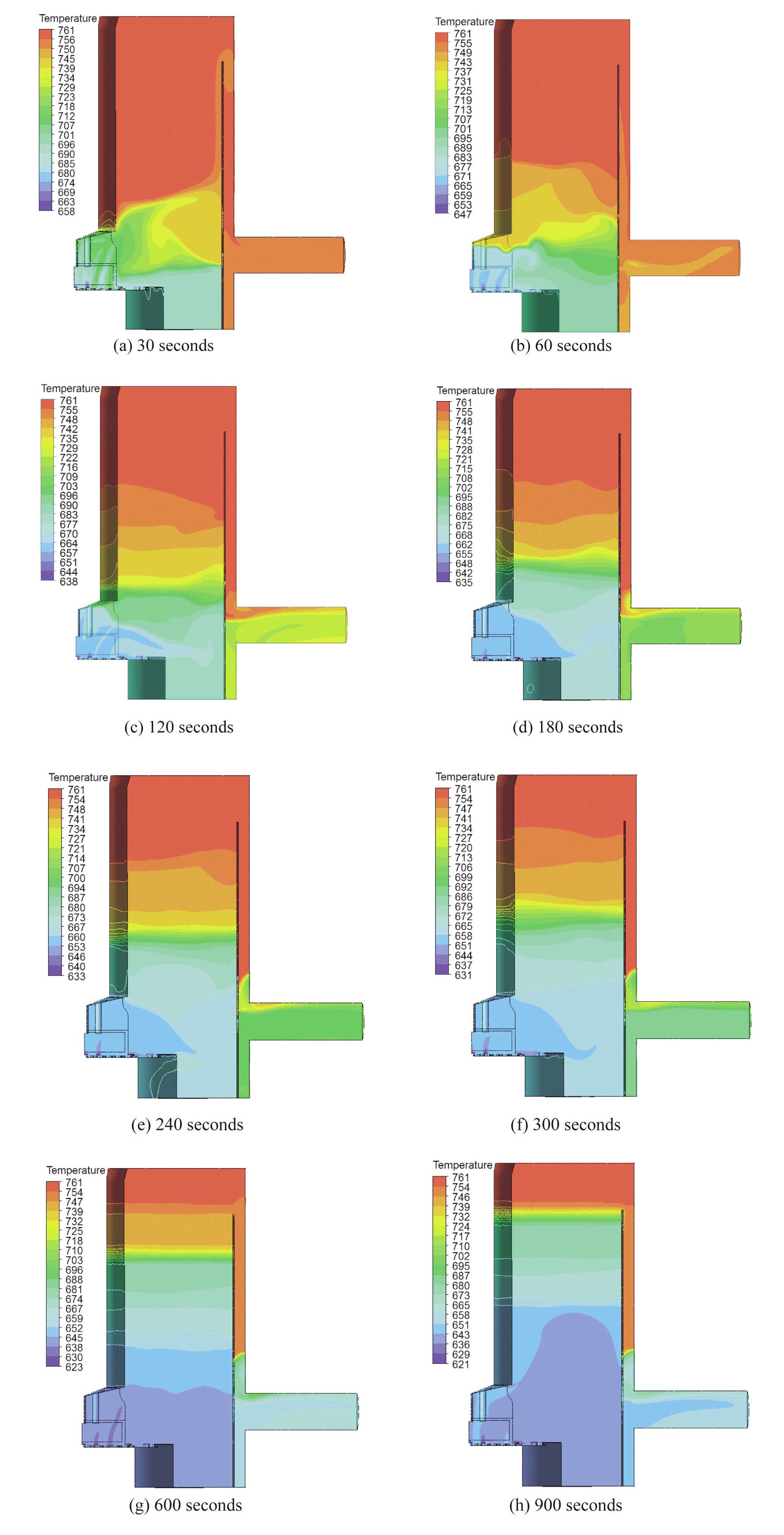
Fig. 8 shows the transient evolution of the temperature field at the upper plenum of the MONJU reactor. When the transient starts and the core outlet temperature gradually drops owing to a reactor shutdown, the cooler sodium stays near the bottom of the vessel and the hotter primary sodium at the higher elevation in the upper plenum stays largely stagnant. As the transient continues, the cold sodium in the lower portion of the plenum moves upward and a thermal stratification begins to form. A rather stable thermal stratification is established at 300 seconds. A slow movement of cold sodium is observed between 240 and 300 seconds. Fig. 7-(a) shows that the rapid coastdown of the mass flow rate after a pump trip is finished at about 300 seconds, and the mass flow rate from the core becomes nearly constant after 300 seconds. Thus, the type of flow until 300 seconds is a mixed convection and the natural convection begins after 300 seconds. At 600 seconds, the thermal stratification interface moves upward rather quickly even though the flow is a natural convection. At 900 seconds, the thermal stratification interface reaches the top of the inner barrel and the temperature field in most of the upper plenum is mixed and homogenized. It shows that a relatively strong thermal mixing has occurred in a large portion of the upper plenum. Thus, the computed temperature field contradicts the real physics of the fluid flow and heat transfer in this region. A stable thermal stratification should form and persist after 300 seconds. The origin of this discrepancy
is due to the turbulence model employed in the present calculation. As explained before, the simple gradient diffusion hypothesis, Eq. (7), for treatment of the turbulent heat flux invokes a relatively strong mixing. A more advanced thermal turbulence model like the algebraic flux model by Hanjalic [6] should be used for a prediction of the thermal stratification; however, such a turbulence model
is not available in the CFX-13 code at present.
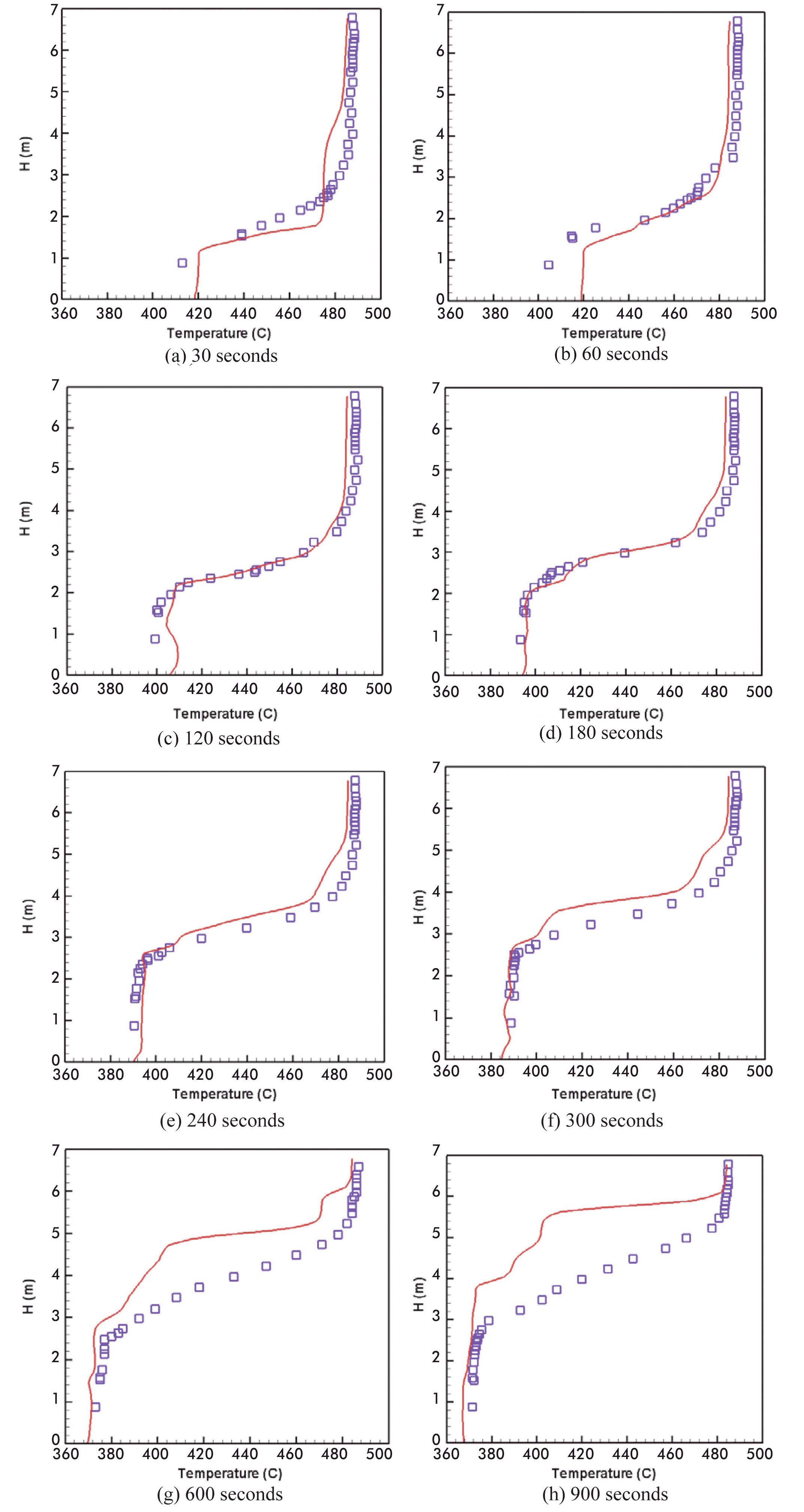
Fig. 9 shows the predicted transient temperature profiles along the thermocouple tree together with the experimental data. It is observed that the predicted temperature profiles agree very well with the experimental data until 300 seconds. However, the predicted results deviate greatly from the experimental data at 600 and 900 seconds. This may be due to the use of the inadequate thermal turbulence model in the present calculation as explained above.
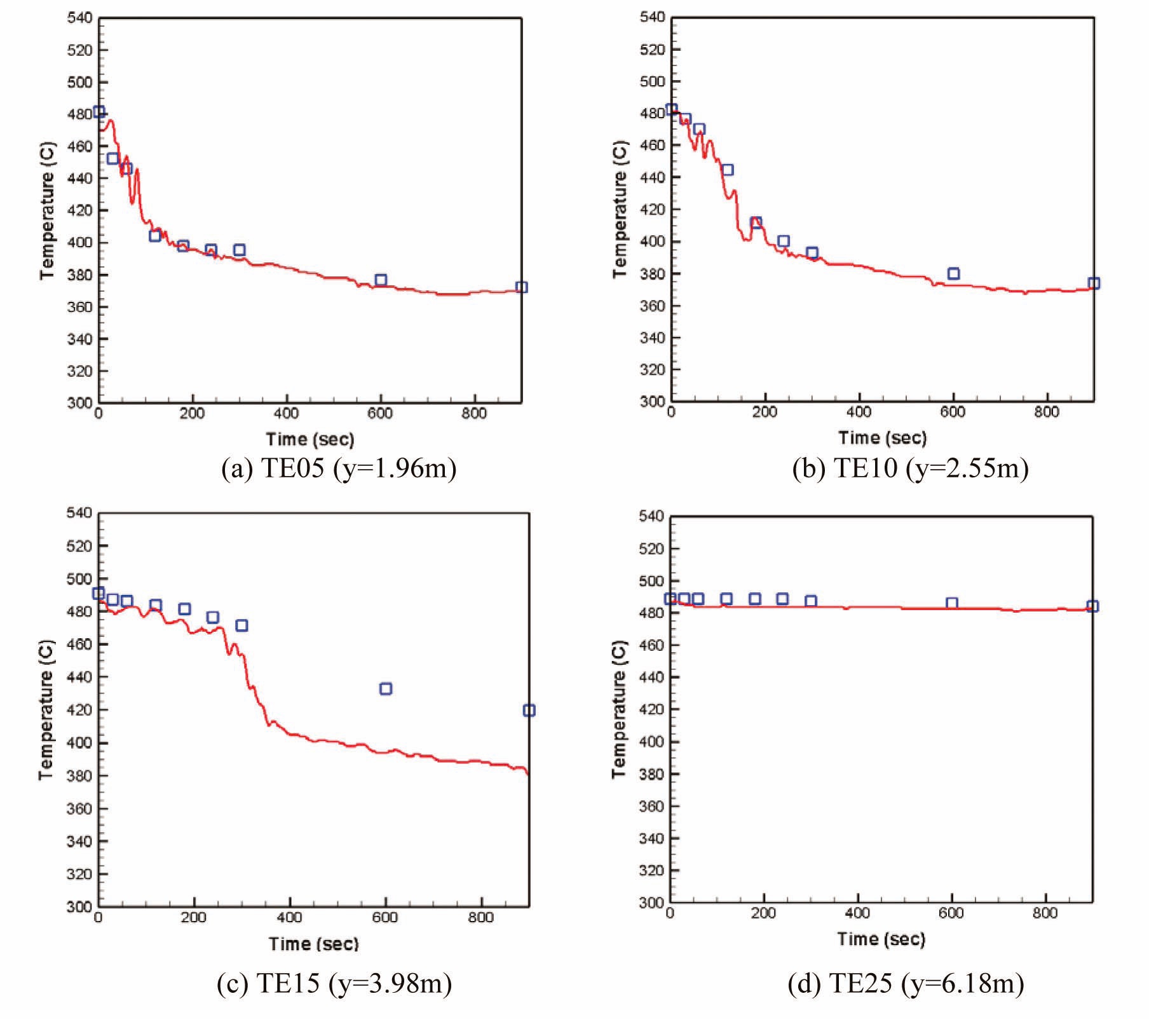
Fig. 10 shows the predicted transient temperature profile at four selected thermocouple locations. The experimental data are available for the first 900 seconds after the pump trip. The agreement of the predicted results with the experimental data is excellent, which is consistent with the results given in Fig. 9.
It is worthwhile to mention that Sofu [19] obtained accurate solutions for the temperature field at 10 and 15 minutes. He employed a round edge flow holes instead of sharp edge flow holes used in the present study. This treatment invokes a small pressure drop through the flow hole and the mass flow rate at the flow holes becomes large. Then, the flow mixing in the upper plenum above the flow hole will be retarded and this makes the resulting solution very much in agreement with the experimental data. The conduction heat transfer through the inner barrel also should be considered with the advanced turbulence models in the future study.
A numerical analysis of the thermal stratification in the upper plenum of the MONJU fast breeder reactor was performed. Calculations were performed for a 1/6 simplified model of the MONJU reactor with a porous media approach to better resolve the geometrically complex upper core structure. A reasonably good agreement with the experimental data was observed for a steady state solution. The results of a transient analysis show that the temporal variations of temperature were predicted accurately in the initial rapid coastdown period (~300 seconds). After the initial coastdown period, the flow type changes from a mixed convection to a natural convection. The simple gradient diffusion hypothesis for the treatment of a turbulent heat flux in the CFX-13 code accurately predicts when the flow is a mixed convection; however, the model invokes a relatively strong mixing for a natural convection flow. Thus, a faster thermal mixing is observed than that shown in the experiment after about 600 seconds. This discrepancy may be due to the shortcomings of the thermal turbulence models available in the CFX-13 code for a natural convection flow with thermal stratification.
a1 : turbulence model constants
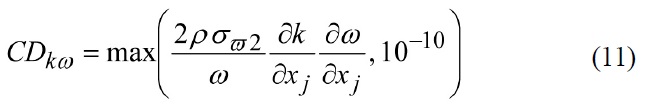
CDkω : turbulence model constant defined by Eq. (11)
Cf : friction coefficient
D : characteristic diameter
De : external diameter
Dh : hydraulic diameter
F1 : blending function defined by Eq. (9)
F2 : blending function defined by Eq. (9)

: frictional force vector
gi : gravity acceleration in -direction
Gk : buoyancy generation term
k : turbulent kinetic energy
K : pressure loss coefficient

: normal direction vector
P : pressure
Pk : generation term of turbulent kinetic energy
Pr : Prandtl number
Prt : turbulent Prandtl number
t : time
T : temperature
Ui : Cartesian velocity components
U : x-directional Cartesian velocity component

: velocity vector

: magnitude of velocity vector
V : y-directional Cartesian velocity component
: Reynolds stresses
xi : Cartesian Coordinates
y : normal distance from the wall
Greek
β : thermal expansion coefficient
β1, β2 : turbulence model constants
β? : turbulence model constant
κ : von-Karman constant
γ : turbulence model constants
ΔP : pressure loss
Δt : time step size
μ : dynamic viscosity
μt : turbulent eddy viscosity
ν : kinematic viscosity
νt : turbulent eddy viscosity divided by density
ρ : density
σk : turbulence model coefficients
σω : turbulence model coefficients

: turbulent heat fluxes
ω : frequency of turbulent kinetic energy
Subscript
ref : pertaining to reference point