Automatic guided vehicles (AGVs) have been a growing research over the last two decades. AGVs have important roles in the design of new factories and warehouses, and in the safe movement of goods to their correct destinations. AGVs have been used in assembly lines or production lines in many factories, e.g., automobiles, food processing, wood working, pharmaceuticals, and other factories. Many researchers have developed and designed AGVs to suit their applications, which are typically related to the major problems encountered in a factory working space.
There are two main types of navigation methods for AGVs: guidance with lines and guidance without lines. In the first type of system, most AGVs track buried cables or guidepaths painted on the floor. One of the most popular types of navigation is based on the use of a magnetic tape as a guide path where the AGV is fitted with an appropriate guide sensor so it can follow the path of the tape [1]. However, it is not easy to change the layout of these guide paths and any breaks in the wires makes it impossible to detect the route. The other form of AGV navigation system uses no paths or guidelines on the floor but instead it is based on laser targets and inertial navigation [2,3]. Vehicles navigate using a laser scanner, which measures the angles and distances to reflectors mounted on the walls and machines. The use of lasers provides maximum flexibility to make easy guidance path changes but this type of system is expensive to construct.
Image processing techniques have also been of interest for detecting and recognizing guide paths during the development of AGVs [4-10]. In many studies related to vision-based orientation, various methods have been introduced for use in navigation systems, e.g., a feedback optimal controller [11], a fuzzy logic controller [12], neural networks, and interactive learning navigation. The use of vision systems has a significant effect on the development of systems that are flexible and efficient, with low maintenance costs, especially mobile equipment. AGV systems that utilize a vision-based sensor and computer image processing for navigation can improve the flexibility of system because more environmental information can be observed, which makes the system robust [13-15].
In this study, we implemented a vision sensor-based driving algorithm to allow AGVs to follow a guide path where markers were installed on the floor, which facilitated high reliability and rapid execution. This method only requires minor modifications to make adjustments for use with any layout platform. Using two cameras, we can reduce the position errors and allow the AGV to change the driving algorithm smoothly while following the desired path. A camera sensor on the top of the AGV can be used to identify the next distant navigation marker. This camera is attached to the vehicle so it subtends an angle
The paper is organized as follows. Section 2 presents the AGV platform configuration. The marker recognition algorithm is described in Section 3. Section 4 explains the driving algorithm for tracking the desired path of an AGV. The experimental results using the two-wheeled mobile robot Stella B2 are given in Section 5, which are followed by the conclusions in Section 6.
This section describes the configuration of the AGV in detail, where a two-wheeled mobile Stella B2 robot is used as the platform, with two 360092305universal serial bus (USB) cameras, vision and movement control software, and a laptop computer.
The Stella B2 robot (NTREX, Incheon, Korea) is a commercial
mobile robot system, which comprises a frame with three plate layers, two assembled nonholonomic wheels powered by two DC motors attached to an encoder, a motor driver, a one caster wheel, a power module, and a battery (12V 7A). A Lenovo Thinkpad (1.66 GHz, 1GB of RAM; Lenovo, Morrisvulle, NC, USA) laptop computer is used as the controller device. The Microsoft Foundation Classes (MFC) control application was built for image processing and movement control. The computer and mobile robot communicate via a USB communication (COM) port.
Two USB cameras are installed on the second and third plate layer. The camera on the second plate layer subtends an angle of 90ο with the floor. The second camera is placed on top of the third plate layer so the angle subtended between its view and the floor is
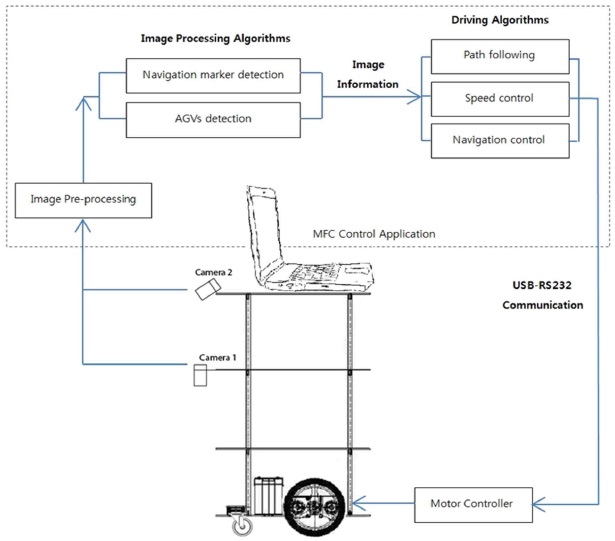
An overview of the AGV navigation control system is shown in Figure 1. The laptop computer obtains environmental information from the front of the robot using two USB cameras. The scenarios analyzed by the image processing algorithm are used as inputs by the driving navigation module so it can set a suitable velocity based on the current AGV environment.
3. Marker Recognition Algorithm
We use markers to provide directional information to the AGV, instead of using the line tracking method. The markers are detected and recognized according to the following steps [16-19].
1) Learn the marker images and classify them using a support
vector machine (SVM).
2) Acquire images from two cameras: camera 1 for a bird’s eye view and camera 2 for a perpendicular aspect.
3) HSV (hue, saturation, and value) color-based image calibration.
4) Noise reduction with median filters.
5) Conversion of binary images
6) Marker extraction using the histogram of oriented gradients (HOG) algorithm.
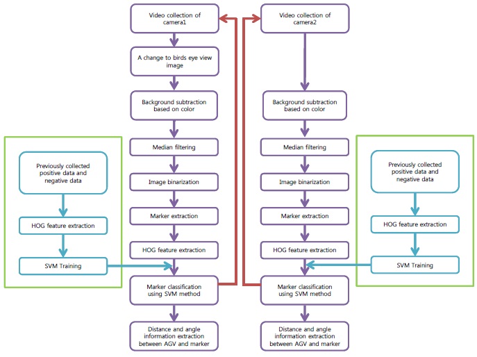
Using the marker recognition algorithm as shown in Figure 2, the markers are detected initially and the directional information and yaw angle information obtained from the detected markers are provided to the AGV. This information is used for AGV path tracking control.
4. Driving Algorithm for Tracking the Desired Path
In this section, we introduce the AGV driving algorithm based on vision sensors, including the movement patterns and the path following algorithm that allows an AGV to track the guide path correctly and robustly while avoiding collisions.
We use five main movement patterns to ensure the smooth performance of the AGV: starting, moving straight, pre-turning, left/right turning, and stopping. The movement pattern changes according to the navigation marker detected by the AGV.
4.1.1 Starting
The AGV does not move forward immediately at high speed but it starts gradually and increases its speed until it reaches the desired velocity. This start process protects the two motors from damage and it also reduces the vibration cause by sudden changes in velocity.
4.1.2 Moving straight
The two AGV wheels move forward at the same speed. When the camera on top of the AGV detects the next straight navigation marker, it increases its speed to the next speed level. If the next marker on the floor is still straight ahead, the AGV will not change its speed. While the AGV moves straight ahead it also uses the path following algorithm to ensure that it remains in the center of the guide path. This algorithm will be described in more detail in the next section.
4.1.3 Pre-turning
The turning marker on the floor is detected by the camera on the top of the AGV. Immediately after its detection, the AGV reduced its speed to a lower rate but it keeps moving forward until the lower camera detects the turning marker. At this point, the AGV automatically changes to the turning pattern. In this movement pattern, the path following algorithm still allows the AGV to keep its exact position on the guide path.
4.1.4 Left/right turning
The AGV reduces its speed continuously and it stops when the center of the AGV is close to the center of the turning marker, before it makes a turn of 90ο from its current position (by maintaining the speed of the two wheels as equal but moving them in opposite directions).
4.1.5 Stopping
Immediately after the AGV detects a stop marker, the overall velocity of the vehicle is reduced so it is equal to zero when the AGV reaches the stop sign. The path following algorithm is also used to drive the AGVs to the correct marker position.
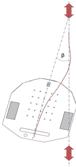
The path following algorithm uses the information the AGV obtains from the vision sensor. The most important information required by the algorithm is the angle between the center of the
AGV and the center of the navigation marker on the floor. The AGV analyzes the angle and gives the two motors an appropriate velocity so it can follow the guide path smoothly and robustly. The upper and lower cameras use this algorithm to ensure more precise path following.
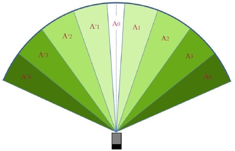
We use nine angle intervals for AGVs, which correspond to nine velocity levels, four angle intervals for turning left, four angle intervals for turning right, and one for moving straight, which track the guide path adequately. The AGV velocity is selected based on the angle between the center of the marker and the center view of the AGV. If the navigation marker is on the center view of the camera or very closed to it in interval A0, the AGV moves straight ahead. However, if the angle between the marker and the camera view center is not in the A0 interval, the velocity of the two wheels will change to make the AGV turn back to the correct track. From angle intervals A0 to A4 or A’0 to A’4, the angle between the AGV and the marker appears to become larger, as shown in Figure 3.
Let us assume that the AGV is in a position, which that subtends angle
Factories often use several AGVs to increase performance. Each AGV works in a different area, but two AGVs or more may work in one area occasionally. To avoid AGV collisions, we constructed a collision avoidance algorithm to protect the AGVs. Based on the information obtained from the two cameras, the AGV can detect whether another AGV is close by, so it can stop moving until the other AGV moves out of the way.
This sections presents our experimental results using a twowheeled Stella B2 mobile robot. Each experiment was conducted in a controlled environment, including the specification of the layout design and the lighting source. The system captured images directly from two USB cameras during real-time, processed the images with the MFC program, analyzed the information using the proposed control algorithms, and sent the result to the mobile robot motor controller via the serial interface of the laptop computer. The overall control system comprised the navigation marker, the AGV detection system, and the driving algorithm. In this experimental study, the control system was evaluated separately according to each of the following criteria: 1) marker detection experiment, 2) AGV detection experiment, 3) path following experiment.
5.1 Navigation Marker Detection Algorithm Experimental Results
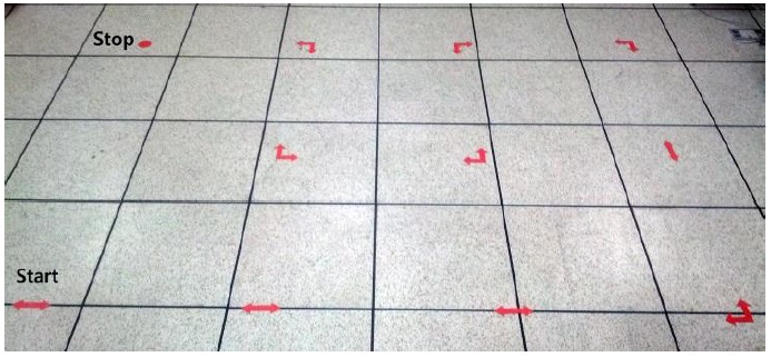
We tested the capacity for autonomous navigations using navigation markers installed on the floor, where the navigation path was set up as shown in Figure 5.
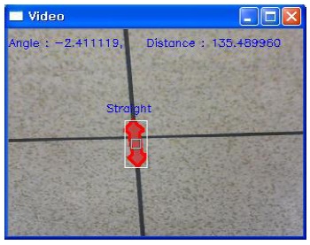
Figure 6 shows a sample image result, which was acquired after the marker detection process. In this image, the marker on the floor is straight ahead, while the negative sign of the angle value indicates that the AGV is deviating to the right from the center of the marker.
The AGVs moved from the start position by detecting the sign marker using the driving algorithm, until it reached the final target.
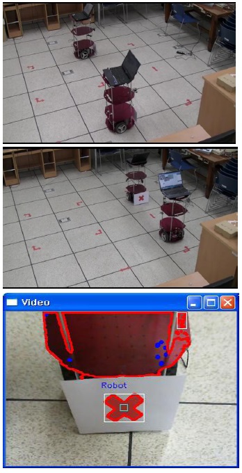
5.2 AGVs Detection Algorithm Experimental Results
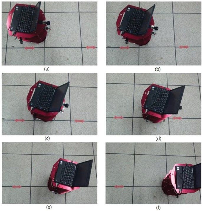
In this experiment, the effectiveness of the proposed AGVs detection algorithm was tested and evaluated using two Stella B2 mobile robots, which moved in opposite directions. When the two mobile robots were sufficiently close to detect each other, they stopped to avoid a collision. Figure 7 shows the experimental results with the AGV detection algorithm.
5.3 Path Following Algorithm Experimental Results
The path following algorithm was constructed to ensure that the AGV would move exactly toward the center of the navigation marker or return to the correct guide path if the AGV was not in the center of the navigation marker. In this experiment, a Stella B2 mobile robot was placed on the floor so it subtended an angle
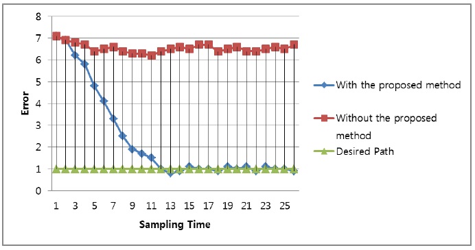
We produced a graph of the path tracking process by generating a log of the angle data while the AGV was running. Figure 9 shows the path tracking control results for the AGV. We compared the path tracking performance of a controller using the proposed driving algorithm with that of a controller that lacked the proposed driving algorithm. Figure 9 shows that the proposed driving algorithm converged on the desired path with 10% tracking errors.
The experimental results showed that the vision sensor-based driving algorithm for AGVs was implemented successfully in a real path guidance system platform in a laboratory environment.
The vision-based marker following method for AGVs worked perfectly using two low-cost USB cameras. The combination of information from two cameras allowed the AGV to operate highly efficiently and smoothly. The AGV followed the guide path correctly and moved as close as possible to the center of the navigation marker using the vision sensors. The AGVs could avoid collisions when more than one AGV worked in the same space. This control system does not require that the destination target is programmed because it depends totally on signs placed on the floor. Thus, AGVs can operate in a flexible manner using any layout.