Feature selection algorithms can be categorized based on
Information theory has been applied to feature selection problems in recent years. Battiti [6] proposed a feature selection method called mutual information feature selection (MIFS). Kwak and Choi [7] investigated the limitation of MIFS using a simple example and proposed an algorithm that can overcome the limitation and improve performance. The main advantage of mutual information methods is the robustness of the noise and data transformation. Despite these advantages, the drawback of feature selection methods based on mutual information is the slow computational speed due to the computation of a highdimensional covariance matrix. In pattern recognition, feature selection methods have been applied to various classifiers. Mao [8] proposed a feature selection method based on pruning and support vector machine (SVM), and Hsu et al. [9] proposed a method called artificial neural net input gain measurement approximation (ANNIGMA) based on weights of neural networks. Pal and Chintalapudi [10] proposed an advanced online feature selection method to select the relevant features during the learning time of neural networks.
On the other hand, the techniques of evolutionary computation, such as genetic algorithm and genetic programming, have been applied to feature selection to find the optimal features subset. Siedlecki and Sklansky [11] used GA-based branchand- bound technique. Pal et al. [12] proposed a new genetic operator called self-crossover for feature selection. In the genetic algorithm (GA)-based feature selection techniques, each chromosomal gene represents a feature and each individual represents a feature subset. If the
In this paper, we propose a feature selection method using both information theory and genetic algorithm. We also considered the performance of each mutual information (MI)-based feature selection method to choose the best MI-based method to combine with genetic algorithm. The proposed method consists of two parts: the filter part and the wrapper part. In the filter part, we evaluated the significance of each feature using mutual information and then removed features with low significance. In the wrapper part, we used genetic algorithm to select the optimal feature subsets with smaller sizes and higher classification
performance, which is the goal of the proposed method. In order to estimate the performance of the proposed method, we applied our method on University of California-Irvine (UCI) machine-learning data sets [14]. Experimental results showed that our method is effective and efficient in finding small subsets of the significant features for reliable classification.
2. Mutual Information-Based Feature Selection
2.1 Entropy and Mutual Information
Entropy and mutual information are introduced in Shannon’s information theory to measure the information of random variables [15]. Basically, mutual information is a special case of a more general quantity called relative entropy, which is a measure of the distance between two probability distributions. The entropy is a measure of uncertainty of random variables. More specifically, if a discrete random variable
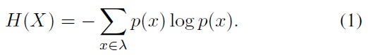
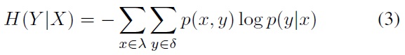
The joint entropy of two discrete random variables
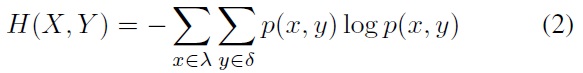
where
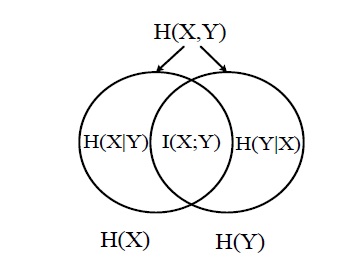
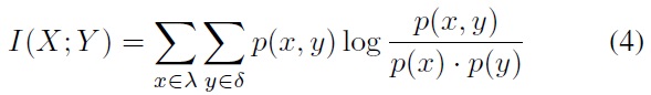
The common information of two random variables X and Y is defined as the mutual information between them:
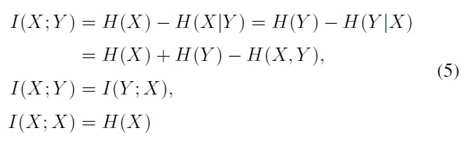
A large amount of mutual information between two random variables means that the two variables are closely related; otherwise, if the mutual information is zero, then the two variables are totally unrelated or independent of each other. The relation between the mutual information and the entropy can be described in (5), which is also illustrated in Figure 1.
In feature selection problems, the mutual information between two variables feature
If the mutual information
2.2 Mutual Information-Based Feature Selection
2.21 Feature Selection Problem with Mutual Information
Feature selection is a process that selects a subset from the complete set of original features. It selects the feature subset that can best improve the performance of a classifier or an inductive algorithm. In the process of selecting features, the number of features is reduced by excluding irrelevant or redundant features from the ones extracted from the raw data. This concept is formalized as selecting the most relevant
Let the FRn-
Given an initial set of
In information theory, the mutual information between two random variables measures the amount of information commonly found in these variables. The problem of selecting input features that contain the relevant information about the output can be solved by computing the mutual information between input features and output classes. If the mutual information between input features and output classes could be obtained accurately, the FRn-
Given an initial set
To solve this FRn-
Typically, the mutual information-based feature selection is performed by sequential forward selection. This method starts with an empty set of selected features, and then we add the best available input feature to the selected feature set one by one until the size of the set reaches
1. (Initialization) Set F ← “initial set of n features,” S ← “empty set.”
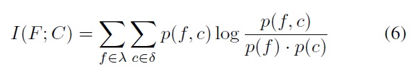
2. (Computation of the MI with the output class) If ∀fi∈ F, compute I(C; F).
3. (Selection of the first feature) Select a feature that maximizes I(C; F), and set F ← F?{fi},S ← {fi}
4. (Greedy sequential forward selection) Repeat until the desired number of selected features is reached.
5. (Computation of the joint MI between variables) If ∀fi∈ F, computeI(C; fi,S).
6. (Selection of the next feature) Choose the feature fi ∈ F that maximizes I(C; fi,S) and set F ← F ?{fi}, S ← {fi}. Output is the set S containing the selected features.
where
2.22 Battiti’s Mutual Information-Based Feature Selection
In the ideal sequential forward selection, we must estimate the joint mutual information between variables
In selecting
cells to compute
Because of this requirement, implementing the ideal sequential forward selection algorithm is practically impossible. To overcome this practical problem, Battiti [6] used only
4) (Greedy sequential forward selection) Repeat until the desired number of selected features is reached.
a) (Computation of the MI between variables) For all couples of variables (
b) (Selection of the next feature) choose the feature
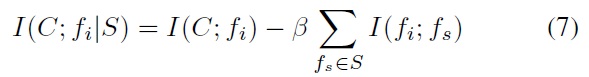
where
3. Genetic Algorithm-Based Feature Selection
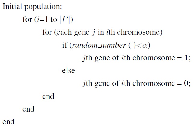
Genetic algorithm is one of the best-known techniques for solving optimization problems. It is also a search method based on a random population. First, genetic algorithm randomly encodes the initial population, which is a set of created individuals. Each individual can be represented as bit strings that can be constructed using all possible permutations in a potential solution space. At each step, the new population is determined by processing the chromosome of the old population in order to obtain the best fitness in a given situation. This sequence continues until a termination criterion is reached. The chromosome manipulation is performed using one of three genetic operators: crossover, mutation, and reproduction. The selection step determines which individuals will participate in the reproduction phase. Reproduction itself allows the exchange of already existing genes, whereas mutation introduces new genetic material, where the substitution defines the individuals for the next population. This process efficiently provides optimal or near-optimal solutions.
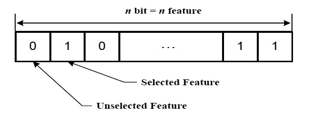
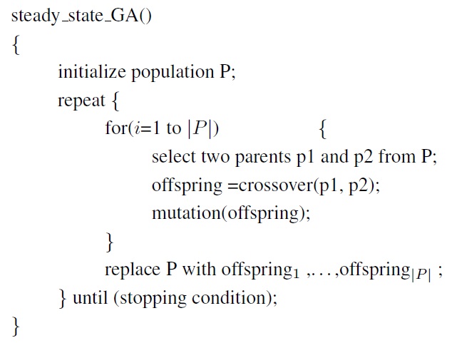
In the genetic algorithm-based feature selection, the size of chromosome
A generational procedure GA is shown below:
4. Proposed Method by Mutual Information and Genetic Algorithm
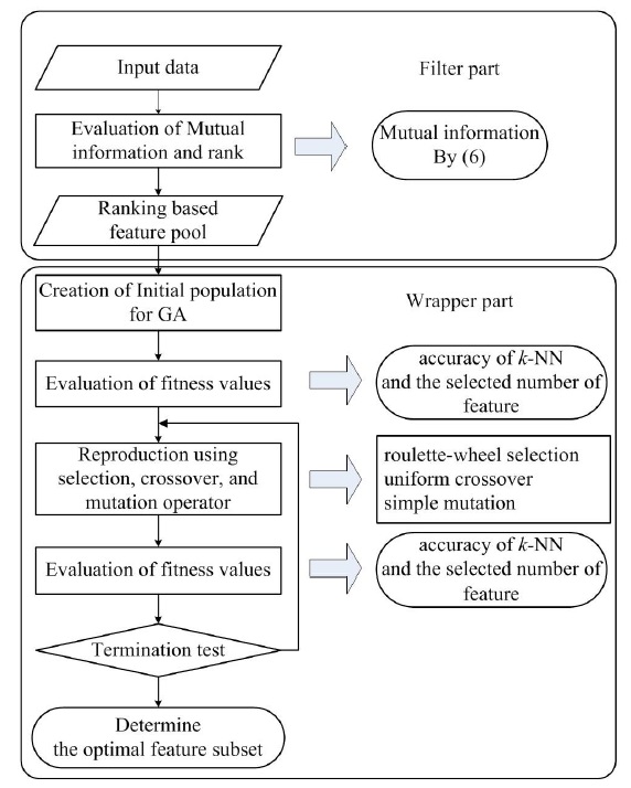
The proposed method can be divided into two parts. The filter part is a preprocessing step to remove irrelevant, redundant, and noise features according to ranking by mutual information. In the wrapper part, the optimal feature subset is selected from the preprocessed features using genetic algorithm with the fitness function based on the number of features and on the accuracy of classification. Figure 2 shows the structure of the proposed method, described as follows.
4.1 Filter Part by Mutual Information
[Step 1]
[Step 2]
high feature size, where
4.2 Wrapper Part by Genetic Algorithm
[Step 3]
An example of a simple procedure is as follows:
where |
[Step 4]
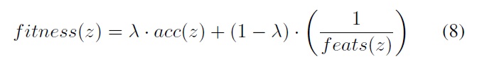
where
where
[Step 5]
[Step 6]
[Step 7]
5. Experiments and Discussions
Ten-fold cross-validation procedure is commonly used to evaluate the performance of k-nearest neighbor algorithm(
[Table 1.] Parameters for the genetic algorithm
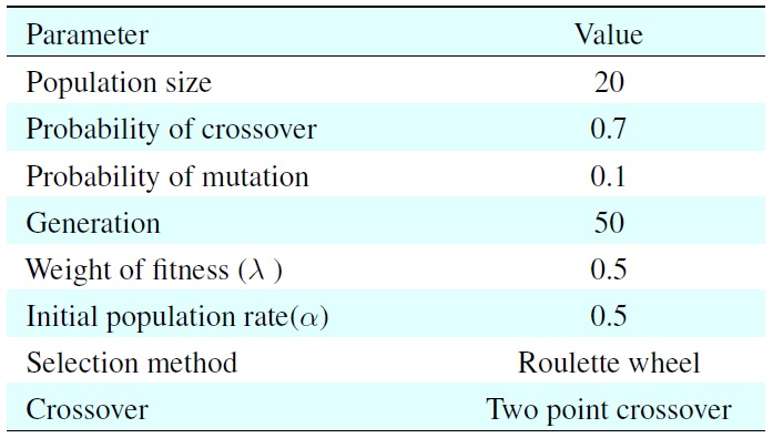
Parameters for the genetic algorithm
the filter part, we used
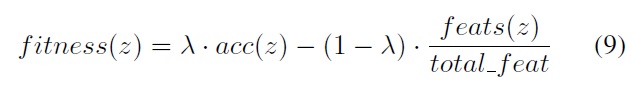
In this experiment, we used the fitness values evaluated by using (9) and the three genetic operators: roulette-wheel selection, uniform crossover, and simple mutation.
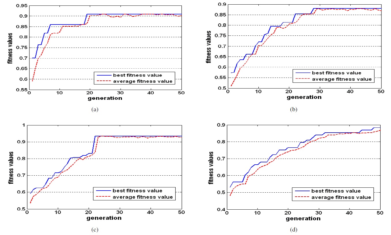
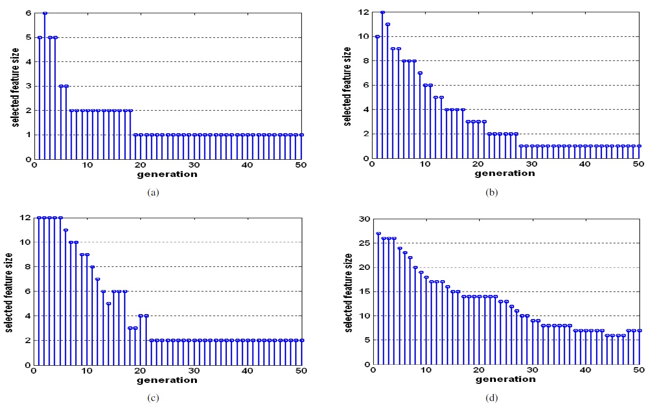
Figures 4 and 5 show the fitness values of GA in each generation and the number of selected features in each generation. We can see that the optimal feature subset was effectively found by the proposed method.
In Table 3, all the results of different methods are obtained from [9]. The NN column lists the results with no feature subset selection. The second column shows the results of the standard wrapper-backward elimination method. The third column shows the results of the ANNIGMA-wrapper method proposed by Hsu et al. The fourth column represents the results of GA, and the final column shows the results of the proposed method. For each error and each number of selected features, we include the average and the standard deviation. As shown in Table 3, the proposed method shows better performance than the other methods for most datasets with small features. More specifically, the error rate is 4.2% when using the eight dominant features chosen bysed method, whereas the error rate is 11.4% for NN without feature selection. From this result, one can see thatsed method makes it possible to dramatically decrease the error.
The feature selection methods can be divided into two groups, filter method and wrapper method, based on their dependence and independence on the inductive algorithm. Filter methods
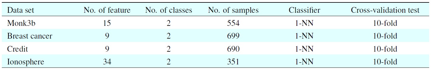
[Table 2.] UCI datasets and classifiers used in this experiment

UCI datasets and classifiers used in this experiment
[Table 3.] Comparison results between the proposed and other methods
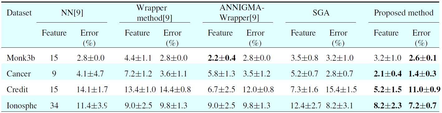
Comparison results between the proposed and other methods
have fast computational ability because the optimal feature subset is selected in one pass by evaluating some predefined criteria. However, they have the worst classification performance, because they ignore the effect of the selected feature subset on the performance of the inductive algorithm. The wrapper methods have higher performance than the filter methods, whereas they have high computational cost.
In order to overcome the drawbacks of both filter methods and wrapper methods, we propose a feature selection method using both information theory and genetic algorithm. The proposed method was applied to UCI datasets and some gene expression datasets. For the various experimental datasets, the proposed method had better generalization performance than previous ones. More specifically, the error rate is 4.2% when using the eight dominant features chosen by the proposed method, whereas the error rate is 11.4% for NN without feature selection. From these results, one can see that the proposed method makes it possible to dramatically decrease the error without increasing the computational time.
No potential conflict of interest relevant to this article was reported