Sound source localization (SSL) is currently a widely researched topic in domains such as human?robot interfaces, diarization, and tracking systems. In this paper, we focus on the online task of multiple SSL.
Using a time-frequency method and a coordinate transformation on the signals received by an equilateral triangle microphone array, we can aggregate direction of arrival (DOA) information from all frequency bins in each time frame [1], giving us a complete set of DOA data for analysis. Because this data will be distributed around the true direction of sound sources, a clustering method can be applied to it to produce SSL information.
In the online task of multiple SSL, the number of sound sources is unknown and changes over time. The data may also contain many highly overlapping clusters and noises, making it difficult to return reliable results. Recognizing this, we suggest that a model-based clustering approach is the most suitable, since nearly all other clustering techniques require the number of clusters ahead of time, or are overly sensitive to noise.
On the other hand, DOA data tends to be distributed in a circular manner. Although mixtures of Gaussian distributions have been used to model DOA data [2], we will demonstrate that the circular distribution of the data makes von Mises (vM) distributions a more natural fit.
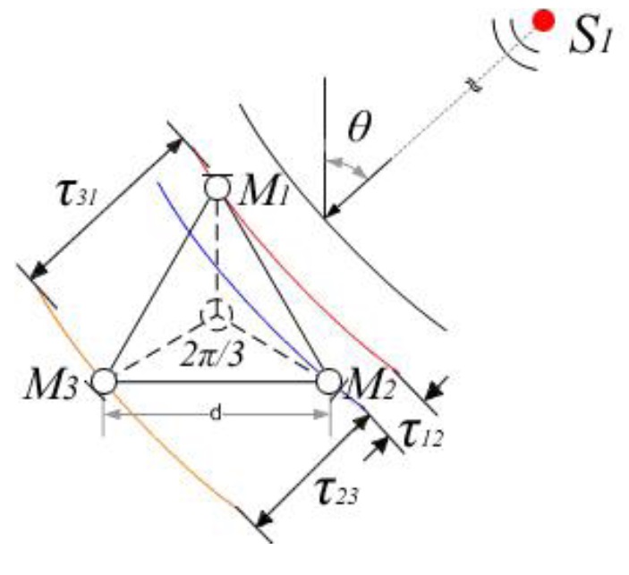
DOA data is estimated using a time-frequency method and a coordinate transformation. The time-frequency method estimates the time delay of signals arriving at three pairs of microphones in a triangle microphone array. The layout of the microphone array is shown in Figure 1.
The time-frequency method is based on two assumptions [3]:
- The sources are disjoint in the time-frequency plane (in other words, at most one source is dominant at a timefrequency slot).
- The distance between microphones is very small compared to the distance between the sources and the microphone array (far-field approximation).
When these asumptions hold, the DOA estimates will be distributed around the true source locations and each cluster in the DOA data will represent a sound source. Note that employing a clustering method can yield an SSL estimation even in an underdetermined case (e.g., when the number of sources is larger than the number of microphones). However, DOA data does have specific characteristics that make clustering challenging:
- It is a kind of circular data, with several features distinguishing it from simpler, linear data.
- It may contain a lot of noise.
- It makes prior knowledge of the number of clusters infeasible.
- Its clusters tend to be highly overlapped.
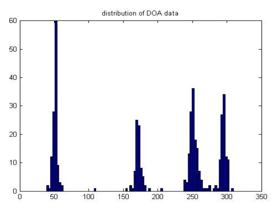
A typical DOA dataset is shown in Figure 2.
Among various clustering algorithms, model-based clustering is the most common approach to clustering analysis because it deals with the problem of determining the intrinsic structure of clustered data when no information other than the observed values is available. In the family of model-based clustering algorithms, one generally selects certain models for clusters and then tries to optimize the fit between the data and the selected models. The EM framework is used to estimate the model with the objective of minimizing the likelihood function of the model.
In circular statistics, the vM distribution is the most popular and natural, much like the Gaussian distribution in linear statistics. Hence, although the Gaussian mixture model (GMM) for model-based clustering provided a classical and powerful approach to clustering analysis in most cases [4], we propose use of the von Mises mixture model (VMM) as the underlying model for DOA data, which are characteristically highly circular. Experiments show that VMM is more effective than GMM in SSL estimation. In [5], the authors provide a generalized EM framework for clustering multi-dimensional directional data on the unit hyper-sphere using VMM. In this paper, DOA data is restricted to two dimensions, so that we need to only degenerate the method proposed in [5] to the 2D case before applying it to our dataset.
Although model-based clustering generally requires the number of clusters as
3. Model-based clustering of DOA data
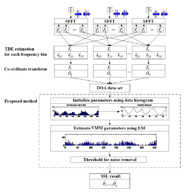
In this section, we will describe the proposed method in detail. The overall workflow of the method is show in Figure 3. The content will concentrated in model-based clustering of DOA data.
In circular statistics, certain basic terms (e.g., mean value, distance) differ from those used in linear statistics. Hence, we cannot apply the distribution functions in linear statistics in the circular domain.
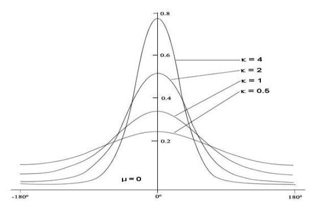
The vM distribution function is commonly used in circular statistics because it has the same merits as Normal Distribution in linear statistics. The vM probability distribution function (pdf) has the form [7]
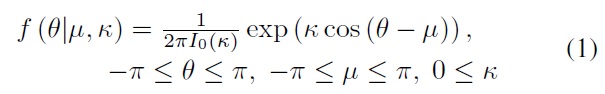
where
3.2 Von Mises Mixture Model with EM Framework
We assume that DOA data can be modeled using a mixture of vM distributions. In [5], the authors proposed a method for modeling directional data on a unit hyper sphere using vM distributions. In our case, the dimensions are only two, so the model can be expressed as
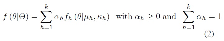
where Θ = {
In this case,
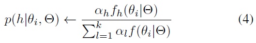
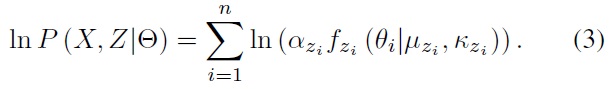
This is the expectation step (E step) in the EM framework. The maximization step (M step) will then re-estimate model parameters Θ to maximize the model likelihood function. There are two strategies for assigning samples to the clusters, suggesting two approaches to re-estimating the parameters in the M step. The two sample assignment strategies are:
- Hard assignment: a sample can be assigned only to a single cluster with the highest conditional distribution (winner takes all). The distribution of the hidden variables is given by
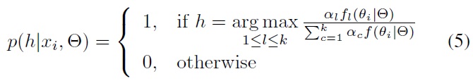
- Soft assignment: a sample can be assigned to many clusters with the probability given by Eq. (4).
The advantage of hard assignment is low computation cost, whereas that of soft assignment is a better fit of model to data. It should be noted that soft assignment can lead to over-fitting problems. In our research, we chose to use the hard assignment strategy due to the time constraints of real-time applications involving SSL detection. Experiments show that even hard assignment can produce good SSL estimations.
In the M step, parameters are re-estimated based on current estimates of hidden variables, according to the following equations:
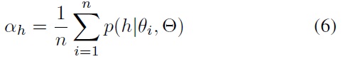
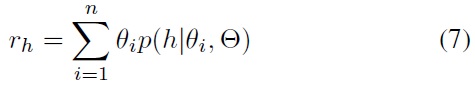
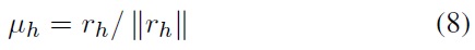

In the above equations,

denotes the sample mean resultant vector. It is used for approximating a concentration coefficient. Note that these estimation equations are 2D simplifications of the equations in [5].
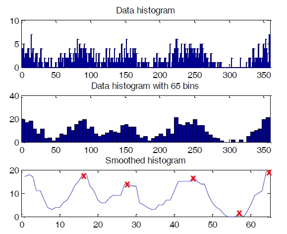
Initial parameters are crucial for model-based clustering. Good initialization of parameters can help the algorithm converge more quickly as well as avoid bad estimations. Since a histogram is a quantized version of the true pdf, we can use it to roughly choose initial parameters for our clustering algorithm. Because the mean of a component pdf strongly corresponds to the location of a histogram peak, we can use the locations of peaks in a histogram as our initial mean directions for the data model. If the dataset histogram is very complicated and yields too many peaks, reducing the number of bins will solve the problem. With DOA data, the degree value of one sample in this dataset can only lie within the range of [0, 360], so a histogram with a number of bins from 36 to 72 is recommended. In our experiment, we used a histogram with 65 bins. The histogram should also be smoothed by a smoothing function such as median filter. After smoothing, we can identify the number of peaks as the number of clusters, and the location of these peaks as the initial values for means directions. Incorrect selections of initial values can be removed using an appropriate threshold after clustering. The steps for obtaining initial values from histogram are shown in Figure 5.
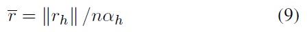
The clustering results of DOA data can contain a lot of clutter caused by noise or reverberation. In estimated models, this type of clutter often appears as low priority (meaning the number of samples belonging to the clusters is small) and low concentration clusters. Thus, we proposed two thresholds for removing such clutter from our clustering results: the
and the
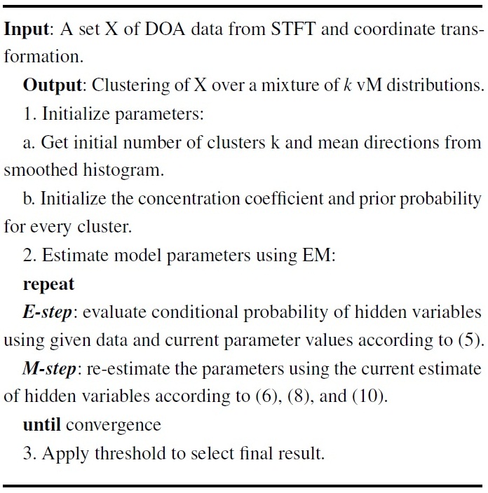
In summary, our method can be expressed by the following pseudo-code:
[Table 11] Algorithm: clustering DOA data using VMM

Algorithm: clustering DOA data using VMM
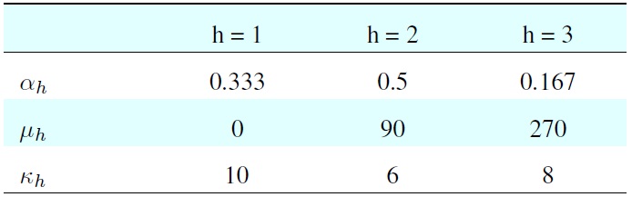
[Table 1.] Parameters for generating the simulated dataset

Parameters for generating the simulated dataset
[Table 2.] Result from model-based clustering of simulated data
Result from model-based clustering of simulated data
4.1 Evaluation of Clustering Algorithm
In order to test the correctness of the proposed algorithm, we tested it against simulated datasets. These datasets were composed by randomization based on the vM distribution.
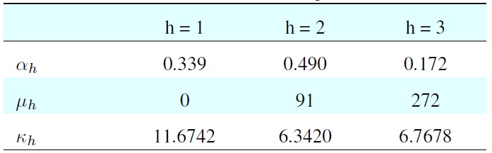
The simulated dataset is composed of highly overlapped clusters randomly generated by the parameters in Table 1.
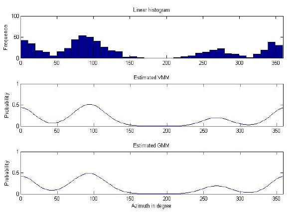
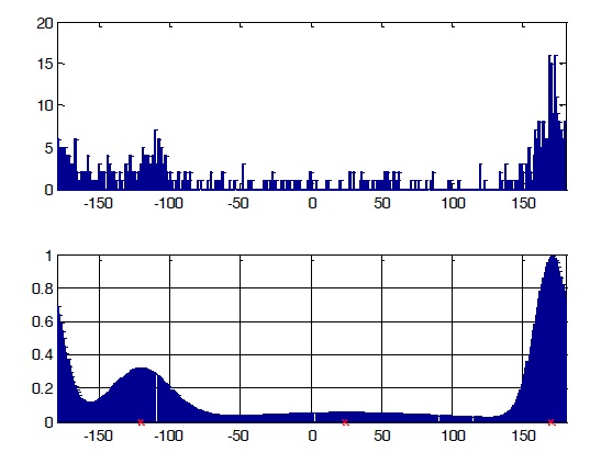
The dataset comprised 600 samples: dataset 1 had 200 samples (33.3%), dataset 2 had 300 samples (50%), and dataset 3 had 100 samples (16.7%). The histogram of input data is shown in the first diagram of Figure 2. The clustering result is shown in Table 2.
In Figure 6, the diagram below the data histogram is the reconstructed model using the parameters estimated by clustering with vMM.
From the result, we can see that the estimation is only slightly different from the parameters used to generate the model. The reconstructed model matches the data histogram closely.
4.2 Experiment on Simulated Dataset
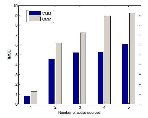
We evaluated the utterances from a TIMIT database, which includes many individual corpora of speech data with durations of approximately 2?3 s. Speech data were randomly selected from the TIMIT database to form a single channel of data. Several of these channels were then passed into a simulated room using the Audio Systems Array Processing Toolbox [8] to obtain mixture signals. We experimented with various numbers of sound sources using both VMM and GMM and compared
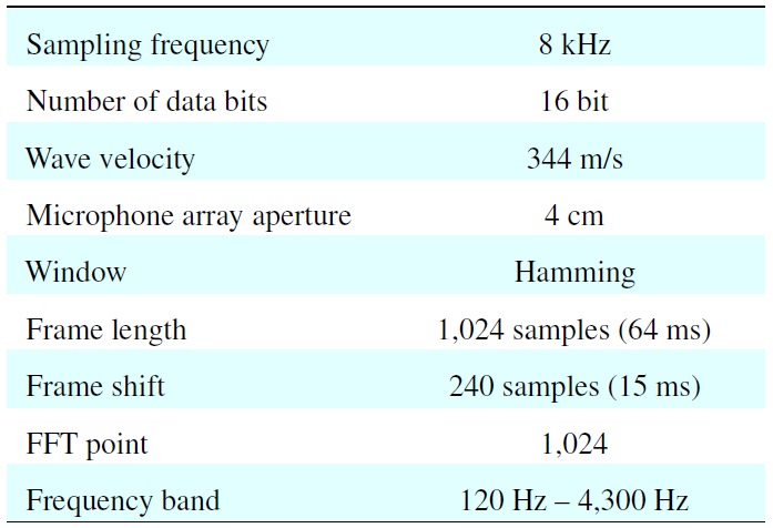
[Table 3.] Parameters for the simulation

Parameters for the simulation
the performances using root-mean-square error (RMSE):
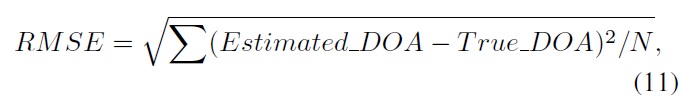
where N is the total number of estimates. The parameters for experiments are set as shown in Table 3. Results showed that VMM worked better than GMM in most of cases, as shown in Figure 7.
4.3 Experiment on RealWorld Dataset
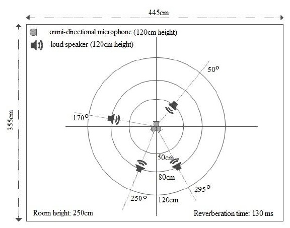
We also performed an experiment to test the performance of the proposed algorithm in the real world. The experimental data for this test was originally used to demonstrate a BSS algorithm in [9]. Four speakers located at directions Θ = 50
A mixture signal is sampled at 8 kHz. A STFT is performed for 1,024 points with a frame of 64 ms (512 samples) and shifted for each 15 ms (120 samples). The bandwidth of the signal is from 60 Hz to 3.96 kHz, resulting in 500 DOA data points in each time frame. The setup of the experiment is shown in Figure 8.
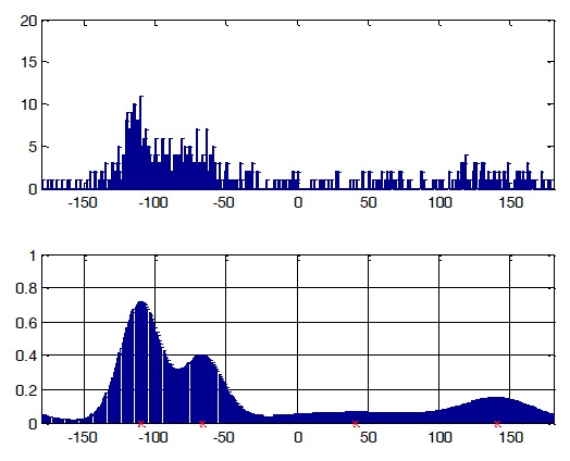
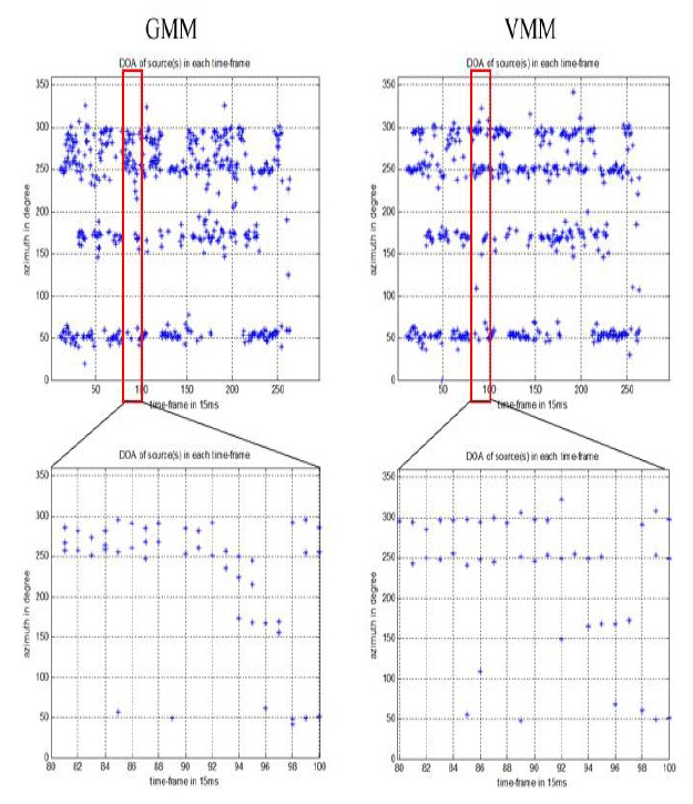
We chose some specific time frames to obtain the detailed results of clustering data from those frames, as shown in Figures 9 and 10. From these figures, we can see that the models estimated using model-based clustering are acceptable for input data, with the number of peaks as our number of clusters and the form of the graph as the initial parameters.
In Figure 11, we see a comparison of the results produced by GMM and VMM for the given dataset at each time frame. It is clear that VMM yielded better results than GMM with respect to both the validity and accuracy of estimates.
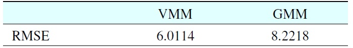
Table 4 shows the RMSE of VMM and GMM for the given
dataset. Note that the proposed method yielded an RMSE of 6.1175 (in degrees) compared to 8.2218 for GMM method.
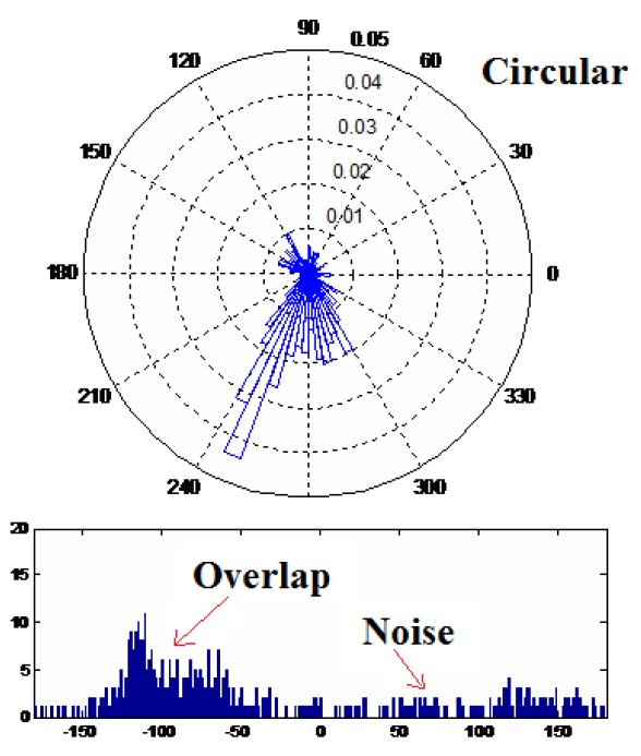
The distribution of results for the entire input signal after applying our noise threshold is shown in Figure 12. From this graph, we can see that there are four sound sources located around the real set-up directions 50
The results of the experiments clearly show that model-based clustering using the von Mises mixture model can estimate the number of sources and their directions with higher stability than the Gaussian mixture model.
The proposed noise threshold effectively removed clutter from the estimated model and added further stability to the estimate. In future work, we will consider a more consistent noise threshold selection method to further reduce estimation errors.
No potential conflict of interest relevant to this article was reported.
[Table 4.] RMSE for VMMand GMMon real-world dataset

RMSE for VMMand GMMon real-world dataset