Transverse magnification (TM) is one of paraxial characteristics of optical systems and is defined as a ratio between the object and image sizes. Unlike effective focal length (EFL) which is an intrinsic property of the system, TM varies depending on the object distance. Because the conjugate relation between object and image distances is governed by the EFL, TM can be expressed in terms of EFL. Thus the relation between TM and EFL can be used as an alternative method to determine EFL by using TM, as for example the so-called reciprocal magnification method used by Anderson [1, 2]. While EFL can be determined by a nodal slide technique as a standard method which requires an infinite light source and an apparatus to locate the nodal point, the reciprocal magnification method requires only measuring the TM at two different conjugations. For finite conjugates, the corresponding TMs are finite and relatively easily measured. Thus, if TMs at various conjugations were measured properly, it would be possible in principle to determine other intrinsic characteristics of optical systems as well as EFL.

The statements in the previous paragraph are based on the paraxial theory. Most real optical systems in finite conjugations are usually suffering from distortion as well as other Seidel aberrations and it is not difficult to foresee the difficulties in measuring properly any characteristics of the system. TM is no exception. Distortion causes the TM to vary along with the object size, which means that the TMs for any finite object sizes are inaccurate. To make matters worse, the amounts of distortion usually depend on the object distance [3]. Thus, without any remedies for distortion, using TM to determine EFL or any other characteristics may not be reasonable.

Conversely speaking, TM would be a useful intermediate characteristic to determine other parameters, if the TM could be measured properly even for the system with distortion. Recently we have developed a method to analyze the distortion for axial symmetric systems [4]. And we found that the method also enabled us to determine TM properly, as we will discuss in this paper. A set of point sources equally spaced in two orthogonal directions is employed and the corresponding point images are analyzed. Provided that distortion is mainly dominant among aberrations, the images consist of the spots corresponding to the point sources in the same orders. During the analysis, the fine alignment for the setup was iteratively searched and the undistorted spot separation along the distortion coefficients can be obtained. Then the TM for the system can be determined from the undistorted spot separation with the separation between point sources.

A thick bi-convex lens system was investigated with a distortion analyzing setup and the TM for an arbitrary object distance was studied. In order to confirm the experimental TM value, we used a set of numerical simulations to match the experimental values. The simulation was carried out by using the finite ray tracing method, and it followed the same experimental procedures. It showed that the method was valid and that the aperture stop’s size along with the defocus of the image plane could be the main sources of the experimental error of a half percent with a moderate experimental configuration.

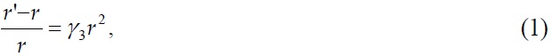
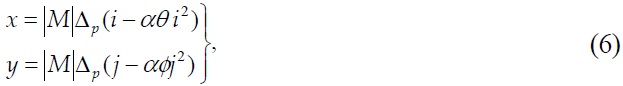
Under the assumption that the lens system under test is axially symmetric, suffering from only distortion, and perfect otherwise, distortion shifts each point of an object radially from the paraxial image point by an amount proportional to the cube of its distance from the center [5], so we define the relative distortion simply as:

where r is the undistorted (paraxial) radial distance for an arbitrary image point whereas r’ is the distorted radial distance for the point from the same origin. The sign of the relative distortion coefficient γ³ defines pincushion distortion as positive and barrel distortion as negative for simple radial distortion. The undistorted image is the scaled object and its radial coordinate can be written as

where M is the transverse magnification and r_o is the radial distance from the origin to the point source. The two origins are assumed to be located on the optical axis. For the point source whose two orthogonal coordinates are given by

where Δ_p is the separation between point sources and the spot numbers (i and j) are integers, the two orthogonal components of the distorted coordinates of the image point can be expressed as

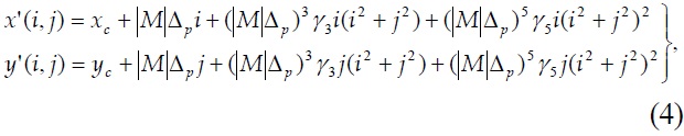
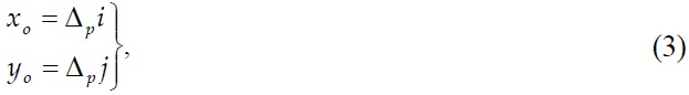
where the origin of the coordinate system is located at the center of the image array (x_c, y_c).

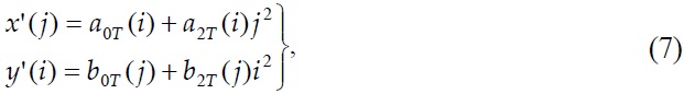
Because of the axial symmetry, Eq. (4) can be simplified for the only spots on two orthogonal meridional planes and their coordinates are given by

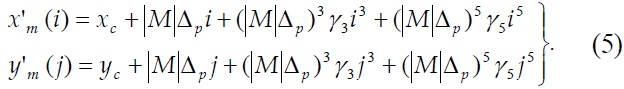
Eq. (5) shows that the coordinates are simply the 3^rd-order polynomials as a function of the spot numbers. Because the spot numbers are integers, the distorted coordinates can be fitted to the polynomial to obtain the best coefficients. The 1^st-order coefficient relates to the separation of the undistorted spots on images and the transverse magnification can be determined with the known value of the separation of the point sources. The relative distortion coefficient can then be determined from the ^3rd-order coefficient.

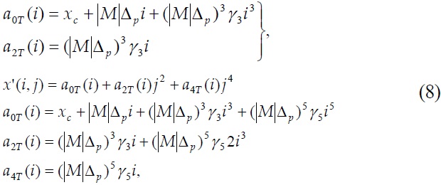
In order to confirm the numerical TM value as well as the distortion, we employed a graph. For the systems, where the relative distortion is only a few percent or less (the case studied in this work), it is not easy to identify the distortion effect from the graph of the distorted coordinates of the spots. So, the constant and linear terms are subtracted from the distorted coordinates in Eq. (5) (hereafter called radial displacement) and it becomes easy to identify the distortion from the radial displacement as a function of spot numbers. In addition, because the radial displacements are the remnants of the distorted coordinates after subtracting the linear and constant terms, it could reveal the existence of the higher order distortion. Thus, if there were higher order distortions, it could be treated simply by adding the corresponding terms in Eq. (4) or (5), accordingly.

The analyzing theory mentioned above is under the condition that the optical axis of the system is all aligned and all planes are perpendicular to the axis, which is not easy to achieve in real situations. Among many possibilities, we considered two cases: the first one is the object plane that is tipped and/or tilted with respect to the optical axis (the tip/tilt axis is passing thru the optical axis) and the second one is the displacement of the distortion center with respect to the axis. The small non-zero angles of tip(？)/tilt(θ) of the object plane with respect to the axis affect the undistorted spot location which can be explained by a pin-hole effect [6] as

where α is a constant parameter related to the image pixel size, distance from the testing system to the image array, and the separation of the undistorted spots. By comparing Eq. (6) and (5), the relative magnitude and sign of the tip/tilt can be identified by the non-zero 2^nd-order coefficient after fitting the coordinates of the distorted spots to the polynomials. The tip/tilt angles can be obtained from the coefficients with the value of the parameter, but it is not necessary because it is important to reduce the angles as closely as possible to zero. The tilted angle can be estimated from the non-zero best fitted coefficient for the distorted horizontal coordinates, while the tip angle from the distorted vertical coordinates in Eq. (5), respectively.

In addition, the non-zero 2^nd-order term displaces the radial displacement curve up or down depending on the sign and magnitude of the angle so that it is possible to identify the existence of the 2^nd-oder term from the graph of the radial displacement as well. This identification in the radial displacement graph can be used to confirm the fitted values for the magnitude and sign of the tip/tilt angles.

The distortion center should be on the optical axis in order to determine the relative distortion coefficient properly. But it is usually displaced from the optical axis with unknown amount because of some reasons, such as tolerance in assembly of camera lens with a detector or the aperture stop being displaced with respect to the axis. The usual approach to determine the amount of the displacement for the distortion center, for example (d_x, d_y) used numerical fitting methods. In the methods, the experimental spot locations were numerically fitted to the displaced coordinates whose origin was displaced as much as the distortion center and the displacements were set as fitting parameters along other parameters. In this study, however, we adopted a different approach. The displacement simply translates all of the distorted spots on an image side to side or up and down, meaning that the distorted spots will be remained in symmetry but the center of the symmetry will be displaced. So, in order to visualize the displacement of the distortion center, we considered the ‘tangential’ coordinates. They are defined as the horizontal (vertical) coordinates of the spots in vertical (horizontal) lines as a function of the spot number of the vertical (horizontal) lines and can be expressed as a set of quadratic equations as:

where

and b_0T and b_2T are similar to a_0T and a_2T, respectively. Equations (7) and (8) show that when the distortion is described by γ³ only, the ‘tangential’ coordinate of the j-th distorted spot on the i-th vertical line can be described as a quadratic function as a function of the spot number, j and the 2^nd-order coefficient a_2T(i), the curvature of the parabolic curve, varies linearly with the spot number, i. Thus, the center of the distortion can be identified as the point where both a_2T and b_2T are zeros and the graph of the a_2T and b_2T as a function of spot numbers will aid the search for the distortion center. Numerically, the center can be calculated by the intercept and slope of the linear function to which the 2^nd-order coefficients a_2T and b_2T are fitted.

The distorted coordinates are the effective results due to the various external parameters as well as to distortion, and we feel that it may not be sufficient to determine every parameter with one measurement. Thus, a set of measurements was iterated to minimize the external parameters as much as possible and when the external parameters are minimized within the experimental uncertainties, the distortion coefficient and transverse magnification were determined.

One additional note is that the 0^th-order coefficients a_0T in Eq. (8) are equal to those in Eq. (5) analytically. This means that the analyzing procedure mentioned above can be confirmed by comparing the fitted coefficients with the actual corresponding spot coordinates on the two orthogonal meridional planes.

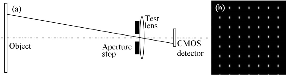
As shown in Fig. 1(a), a 15” LCD monitor (pixel pitch = 0.294 × 0.294 mm²) was used as an object plane to display a number of bright pixels in a square grid (55 × 55) as point sources and a circular aperture of diameter 3 mm was placed in front of a bi-convex testing lens (BICX-25.4-23.9-C, CVI Melles Griot, f=24.8 mm at λ = 546 nm). The aperture stop was placed as close as possible to the lens. The distance from the monitor to the aperture was measured coarsely and it was 327.5 ± 0.5 mm. Among RGB colored pixels, only green pixels for the point sources were turned on with maximum intensity (=255 intensity) and all other pixels were turned off (=0 intensity). The spectrum of the light was measured and the wavelength of the green light was found to be 544 nm. Images were measured with a CMOS camera (Mightex Systems) and the detector pixel pitch was 5.2 × 5.2 μm². Fig. 1(b) presents a typical image cropped from the original size (1024 × 1024) to the 141 × 141 in the central area. The camera was positioned at the best focus location, where the averaged peak intensity of the several spots in the central area was maximized.

Each of the 4 elements (monitor, aperture, lens, and the camera) was mounted on a xyz-translation stage whose precision is 10 μm independently from each other in order to maximize the degree of freedom to adjust. In addition, the monitor has two additional adjustments for tip and tilt angles with the same type of micrometers. The brightness or gain of the camera was adjusted so that the maximum intensity (including the background noise) of the spots in images was under the saturation level. In order to acquire an image, a set of 100 frames was averaged with all the pixels on the monitor being turned off and another set of 100 frames was averaged with the pre-chosen pixels on the monitor being turned on. The first set of frames was regarded as background noises and was subtracted from the second set of frames in order to optimize the spot location analysis for each image.

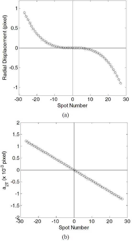
The coordinates of the spots in the image were determined by using a center of mass algorithm. The center spot and four nearest neighbor spots were centroided and the remaining spot locations were searched and determined based on the information of the 5 spot coordinates. A set of fitting procedures, described in Sec. II, was performed using all the coordinates of the spots in the image. Fig. 2 shows the radial displacements of the two orthogonal meridional planes (red-vertical; blue-horizontal) and 2^nd-order coefficients a_2T (red) and b_2T (blue) of the tangential coordinates, respectively for the image shown in Fig. 1(b).

Figure 2(a) shows that the distortion is about 1 pixel shorter (barrel distortion) than the paraxial location for the 27-th spot (about 496.6 pixels away from the distortion center) and it means that the relative distortion is about -0.2 %. The radial displacements for the horizontal (blue) meridional plane in Fig. 2(a) are almost symmetric, while those for the vertical (red) plane are displaced slightly upward, indicating that the object plane (monitor) is slightly tipped. The overall experimental error for the tip/tilt angles of the monitor was equal or less than 0.1°. The 2^nd-order coefficients shown in Fig. 2(b) are almost zero at the 0^th-spot number and the experimental error for the distortion center was close to the optical axis at about 0.02 mm. Even though the magnitude of the tip/tilt angles and the amount of the distortion center displacement were not exactly zero, the effect due to these errors on the final determination was found to be negligible. After a series of measurements to minimize the tip/tilt angles and aligning the distortion center to the optical axis, the image shown in Fig. 1(b) was collected. The spot separation in this image was found as 18.357 ± 0.007 pixels. The uncertainty of the spot separation was measured over a number of trials and was found to be less than one hundredth of a pixel. As the separation between the green pixels on the monitor was 1.176 mm (=4 × 0.294), the transverse magnification was -0.08117 (=-(18.357 × 0.0052)/1.176).

To confirm the value of the transverse magnification, a set of numerical simulations was performed for the system configured numerically to be as similar as possible to the

actual setup, as shown in Fig. 1. The main computation was to trace the rays from a set of point sources on an object plane by finite ray tracing [5] to the image plane. The program was written using Matlab software [7]. The computation was performed once the numerical coordinates of the intersecting points of the rays at the image plane were confirmed to be correct with those calculated using the lens-design software [8]. The distance from the object to a bi-convex lens and from the lens to the image plane were set to 327 mm and 23.28 mm (from the lens to the paraxial image plane=23.286 mm), respectively. The aperture stop was in contact with the lens, the refractive index for the lens was set as 1.51873 for λ = 546 nm. The center thickness and radius of curvature of the lens were measured to be 9.95 and 23.9 mm, respectively [9]. A set of point sources in a square grid (55 × 55 = 3025) on an object plane, which were separated by 1.176 mm orthogonally, was considered and a set of rays (201 × 201 = 40401) emerging from each point source was numerically traced to the image plane through the circular aperture stop of 3 mm in diameter.

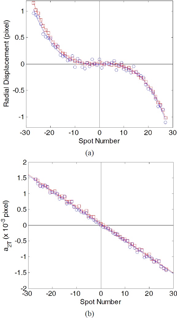
The intersecting points of the rays from each point source with the image plane were averaged and the two orthogonal coordinates of the set of averaged points were regarded as the spot coordinates from the actual images and analyzed by the same method, described in Sec. II. Fig. 3 shows the radial displacement and 2^nd-order coefficients a_2T for the simulated system. The system was assumed to be all aligned in a perfect condition. Both radial displacement and 2^nd-order coefficients of the tangential coordinates agree well with the experimental correspondences shown in Fig. 2. In addition, the simulated spot separation is 18.355 pixels and the transverse magnification is -0.08116, which also agree well with the experimental values of 18.357 pixels and -0.08117, respectively. The paraxial transverse magnification is -0.08112 based on the paraxial ray tracing

for the system with the Gaussian image plane.

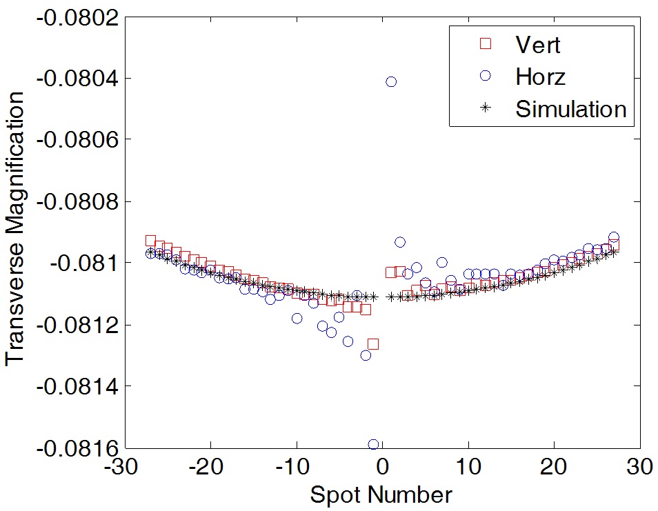
In order to demonstrate the effect of the distortion on transverse magnification, the image spot locations were simply divided by the corresponding point source locations in two orthogonal meridional planes and they are shown in Fig. 4. The black star symbols in Fig. 4 correspond to the same results for the simulated image. The magnitude of the magnification was decreased as the spot number increases because of the barrel distortion; the farther the point source gets away from the optical axis, the more magnification deviates from the paraxial value. Even though it was not possible to obtain the magnification value at the 0 spotnumber because the source was on-axis, the distortion analysis could provide the paraxial value of -0.08116. It is noteworthy to see that the magnification values shown in Fig. 4 are noisy near the distortion center, indicating that a simple division of the spot separation near the distortion center by the point source separation does not guarantee the proper determination of the transverse magnification because of the noises in the image measurement..

Even though the transverse magnification (-0.08116) obtained for the simulation agrees well with the paraxial transverse magnification (-0.08112), they still are not equal to each other. Thus, we repeated the same simulation with a different size of the aperture stop and the transverse magnification becomes -0.08113 when the aperture stop is 1 mm in diameter and the image plane is at 23.286 mm from the lens. This means that the transverse magnification can be affected by not only the image plane location but also by the aperture stop size. With more simulations, we found that the aperture stop size was causing more error than the image plane location. If the intensity of the light emitted by the monitor’s pixels were brighter, the aperture stop size can be reduced and the more accurate value for the transverse magnification can be expected. In addition, the brighter sources can also reduce the signal to noise ratio and it will enhance the determination.

We have demonstrated both experimentally and numerically that distortion analysis enabled us to determine the transverse magnification of imaging systems. Because the transverse magnification can be determined accurately, other characteristics of the system can also be determined by using the transverse magnification, in principle. Some studies are in progress currently [10,11].