A stable energy supply is indispensable for human life, given the fact that energy demand has been sharply increasing because of rapid industrial expansion. Extensive piping facilities are used in heat power plants and nuclear power plants, which supply most of the energy worldwide. Hence, there is a need to develop a system for avoiding breakage of pipes in piping facilities and to perform precise inspections of power facilities for defects to ensure a stable and continuous energy supply. When piping facilities involve extensive use of pipes and pressure vessels, defects from corrosion will be a common occurrence in such facilities. Such defects may often remain unnoticed until some destruction has been occurred [1].
The current techniques used for preventing such defects are ultra waves (microscopic defect detection and rapid detection is possible, but shape and internal structure of the product can affect the test), x-rays (can be applied for all materials with different thickness defect detection but radiation safety management is challenging. More than 15 degrees rotated cracks cannot be detected and it is difficult to detect microcracks), and eddy currents (generally used for detecting defects in nonmagnetic materials and in the case of a magnetic object, identification of a defect is difficult because of residual magnetism). Although people use various ways to detect defects, there are different problems with the contact method, mainly lack of proper methodology and skill. Hence, to overcome these disadvantages, we have used the ESPI method in this work. The advantages of an ESPI system include rapid measurement, high accuracy, and non-destructive and non-contact inspection. Owing to such advantages, the ESPI method is assumed to stand above existing measurement methods across all industries. This optical method has been recently discussed regarding its use across many industries where they use non-destructive testing in their techniques [2].
An electronic speckle pattern interferometer can be classified, on the basis of the type of deformation that it can measure, into in-plane and out-of-plane. It can also be classified on the basis of the lengths of its components and the shape of its optical components: a bulk-type and an optical-fiber type. Bulk-type ESPI of the optical configuration is complex and susceptible to outside influences (sensitive to light and vibration) [3]. Bulk-type ESPI is difficult to apply in the industrial field. In this study, we focused on the accurate measurement of defect length by using an optical-fiber-type ESPI. By preferring the optical-fiber-type ESPI over other ESPIs, we gain the following advantages; (1) It is cheaper than bulk-type ESPI (2) it is very simple to set up (3) there is no restriction on the type of material to be measured (4) complex components of existing measurement systems can be remodeled easily, and (5) it is less affected by disturbance and vibration than the bulk-type system [3,4,5].
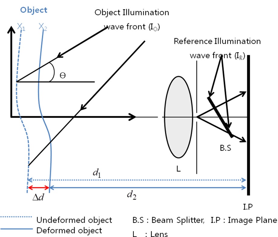
We measured out-of-plane displacements by arbitrarily selecting two wavelengths that are superimposed on each other. Their condition, before and after the deformation of the specimen, is recorded through their four fringe images which are taken before and after their deformation by an external force [6,8]. The intensity of light, before the object is deformed by the force, is given as follows:

In this equation, IO is the amplitude of the object beam and IR is the amplitude of one of the reference beams.

where,
The phase difference in the object beam before and after the deformation takes place is expressed as follows:

where d1 represents the degree of deformation of the object in the direction of the wave front, d2 is the deformation in the X2 direction, and λ is the wave length of the laser. Thus, the degree of deformation is expressed as follows:

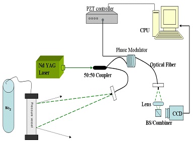
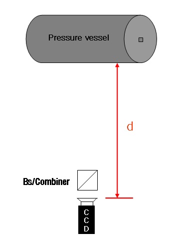
In this study, the method used for experimentation is the optical- fiber system which uses principles of out of the plane ESPI as shown in Fig. 2. The optical-fiber system is arranged on an optical table, which does not require protection against dust because it is not very sensitive to vibration and disturbance. A 532 nm CW diode-pumped solid-state (DPSS) laser obtained from Cobolt Samba is used as a light source. The intensity of the laser was approximately 150 mW. We used an optical-fiber system (Thorlabs Co.) having a dimension of 1 m × 2 m.
The permitted limit of the specific wavelength is between 532 and 640 nm and the laser beam emitted by the laser is divided into an object beam and a reference beam using a coupler with 50:50 magnifications. The object beam is emitted directly to a pressure vessel. The beam emitted to the pressure vessel enters a charge-coupled device (CCD) camera after reflecting from the surface of the pressure vessel. Then the reference beam is focused, and emitted into the CCD camera. The reference beam is controlled by a PZT cylinder, PT-130.14, obtained from Pi Co. An optical fiber is wound twenty times around the cylindrical
phase modulator, whose thickness can expand up to ±16 μ m when maximum voltage is applied. Thus the intensity distribution by interference is stored in a frame grabber through the CCD camera [7].
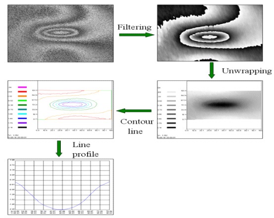
The frame grabber installed on a computer converts an analog signal to a digital one, and we used a frame grabber in our work because the data entered through the CCD camera was an analog signal. Interference fringes appear on the monitor after each of the eight images are extracted (four images, each captured both before and after deformation). They are saved on the image grabber. Eventually, the monitor displays a complete phase map according to the information of the displacement gradient using an equation that can estimate a value for the reference beam phase that is modulated four times using the PZT controller. Eventually, phase modulation to obtain a 4-bucket (4-step) algorithm uses PZT. Using the phase map obtained in this manner, we can understand the defect formation and estimate the displacement value [9,10].
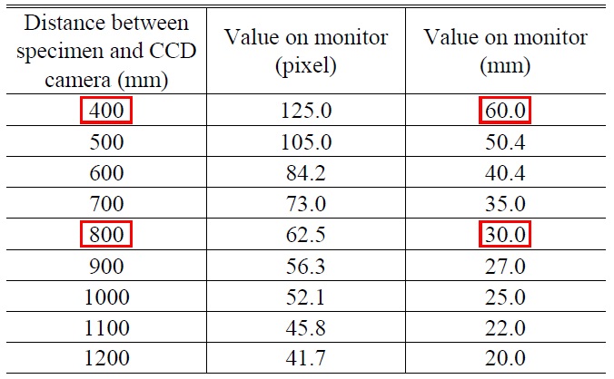
Out-of-plane deformation can be measured from the fringe pattern by phase. The size of the fringe pattern can be used as a measure of internal defect length. For quantitative measurement of the defect length, the size of the fringes that appears on the computer monitor should be known. Table 1 lists the lengths of fringes on the screen according to the distance between the specimen and the CCD camera. Calculations should be done in pixels in order to measure these lengths quantitatively. In the 15-inch monitor used in this study, 640 pixels exist on a 12-inch width. Hence, on our monitor, 1 pixel was equivalent to 0.48 mm. For example, Fig. 3 shows that when the distance between the specimen and the CCD camera is 80 mm, an actual length of 30 mm appears to be 30 mm on the monitor.
However, we selected a distance of 400 mm, which appeared as 60 mm on the monitor. In other words, the ratio of the actual distance to that appearing on the monitor is 1:2 (CCD 400 mm is 60 mm in monitor/ CCD 800 mm is 30 mm in monitor). To reduce error with decreasing distance, we took each measurement 2 times.
[TABLE 1.] Fringe lengths according to the distance at a length 30 mm

Fringe lengths according to the distance at a length 30 mm
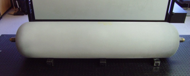
The specimen shown in Fig. 4 is made of aluminum 6061-T4 (Modulus of elasticity = 68.9MPa, Poisson’s ratio = 0.330, Density = 2.70 × 10⁻⁶ kg/mm3). In our experiments, we used an aluminum liner which was a component of CNG fuel tanks used in buses as the specimen. The length, external diameter, and thickness of specimen were 1540, 356, and 5.5 mm, respectively. Both ends of the specimen had screw threads which could be used to attach a cab that is used to apply the pressure to the specimen on the device. We can supply compressed gas to the specimen by creating a hole through the center of the cab. The surface of the specimen was painted white so that the aluminum liner could uniformly reflect an emitted laser beam. The internal defect in the specimen was circumferential having a depth of 3 mm, and varying lengths of 10 mm, 20 mm, and 30 mm. To estimate the defect length, we used electric-spark machining to artificially create a defect inside the aluminum liner [9,13].
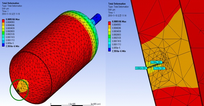
Figure 5 shows the finite element analysis of the specimen. To ensure system stability during a pressure test, we used the simulation program ANSYS Workbench v.10. Mesh type was tetra mesh and element size: 10 mm, the number of node: 90317 and element: 45947, material: aluminum alloy, analysis type: linear static analysis. To perform accurate measurements, the test pressure should not exceed the maximum allowable pressure. In our research, the displacement
of a defect in the pressure vessel was measured for a maximum pressure of 0.070 MPa and minimum 0.014 MPa. As shown in Fig. 5 the displacement of the defective part in the pressure vessel was about 0.0004 μm, and this value did not affect the estimated values.
To analyze phase map data quantitatively, we used ESPI measurement equipment which is available commercially. It is called Q-100 Micro-star equipment, and it is used to measure small displacement. We used ISTRAMS 2.4.2 (4-bucket image processing analysis unit) to capture images of the defects to identify their shapes.
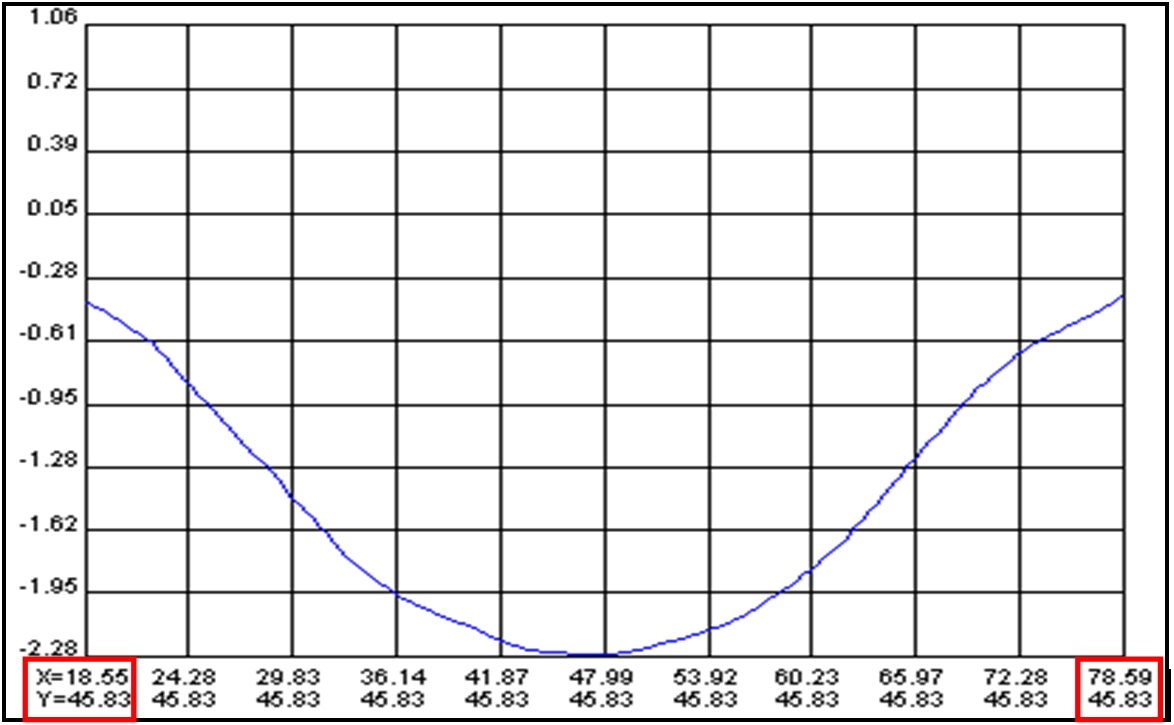
Through operation, we obtained a contour line with their standardized maximum and minimum. From the line profile data, we estimated the values of defect length using subtractions along the X-axis, as shown in Figs. 6 and 7.
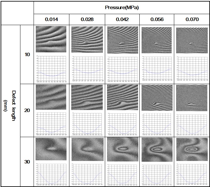
Figure 8 shows the experimental results which indicate the phase map for the case of an axial flaw in the circumferential direction with a defect depth of 3 mm and three different defects lengths of 10, 20, and 30 mm using the optical-fiber ESPI system. The measurable laser-beam irradiation area is 144 mm × 110 mm and the intensity of the laser used in these experiments was 150 mW. We used a pressurizing method that input nitrogen gas into the pressure vessel to produce a deformation.
We applied a pressure of 0.014, 0.028, 0.042, 0.056, and 0.070 MPa on specimens with three different defect lengths. To achieve accurate results, a pressure of 0.070 MPa was determined as the maximum pressure. If the pressure exceeded its maximum value, the interference fringe would have appeared overlapped with other fringes.
In this study, values of the defect length were estimated in the line profiling step in the four-step image processing
[TABLE 2.] Estimated defect lengths for pressure of 0.070 MPa
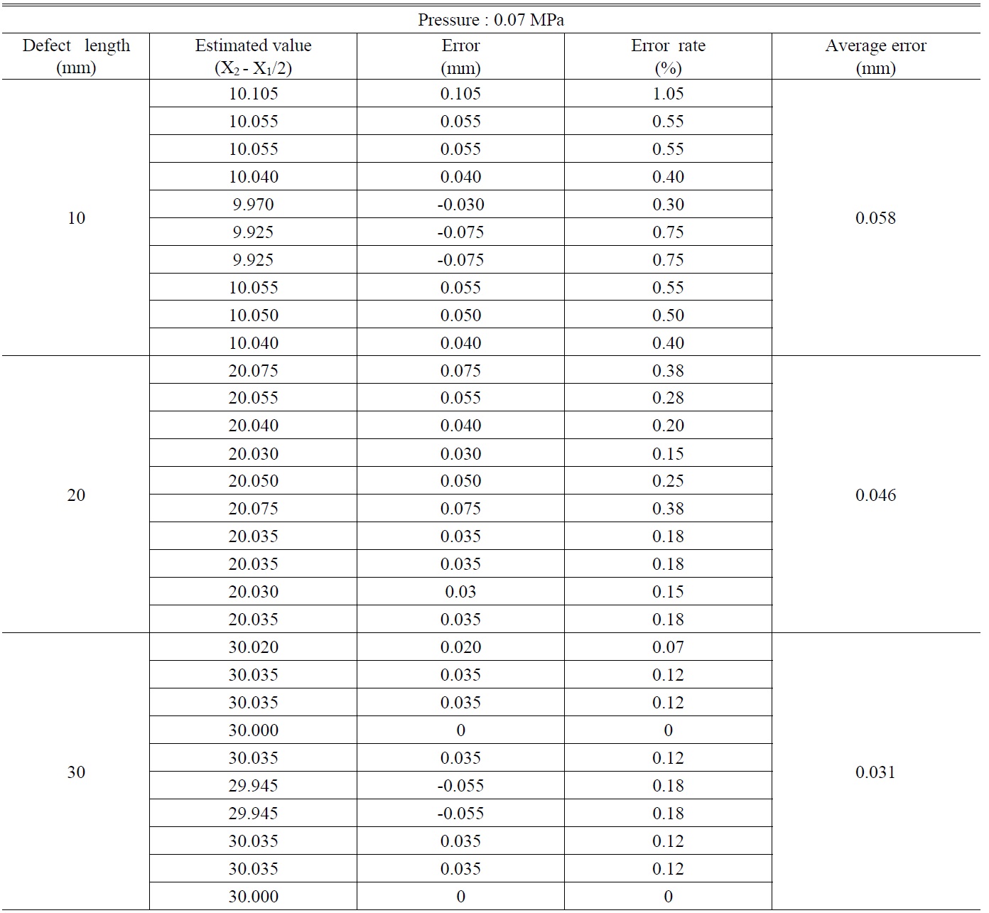
Estimated defect lengths for pressure of 0.070 MPa
equipment obtained from Microstar. This is a way to use maximum values and minimum values for the horizontal axis of the line profile. Through this study, our aim was to confirm the reliability of the proposed systems for accurately measuring defects inside the aluminum pressure vessels, as done in the case of the experimental specimen made of carbon steel.
To confirm the reliability of our proposed system, we compared and analyzed actual values with the estimated values. We performed experiments using the optical-fiber ESPI system over ten times. It should be noted that it is difficult to obtain a proper phase map that can provide the information about the defects inside a pressure vessel made of carbon steel under pressure conditions of less than 0.280 MPa.
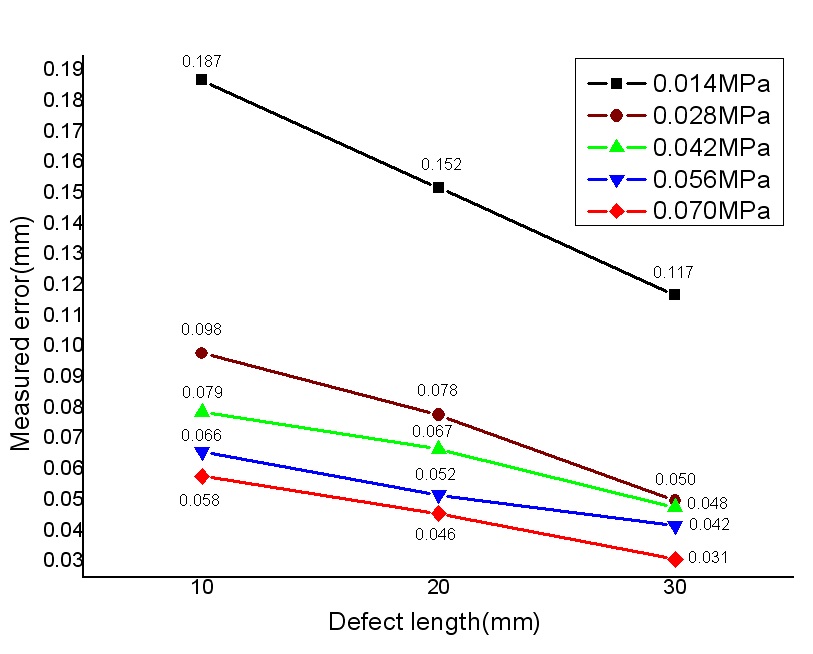
However, we obtained a good phase map for the defects on the aluminum liner at a substantially low pressure of 0.014MPa. A slightly larger error rate was estimated when the defect length and applied pressure were 10 mm and 0.014MPa, respectively. However, it should be noted that as the defect length and applied pressure increased, the estimated values became remarkably consistent with the calculated one. Table 2 shows the values of defect lengths at a pressure of 0.070 MPa. The average errors for defect lengths 10, 20, and 30 mm are 0.058, 0.046, and 0.031 mm, respectively. This proves that the defect length increases with decreasing error rates. Fig. 9 shows a graph of the calculated values of defect lengths according to the pressure variation.
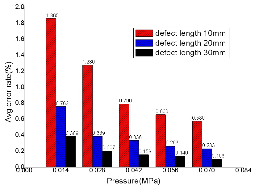
In other words, the higher the pressure, the more the defect length error has been decreased. Fig. 9 is the average error rate; Fig. 10 showed the same pattern.
Our study proved that by using an optical-fiber ESPI system, it is possible to quantitatively measure the length of a defect on an aluminum liner used in composite pressure vessels. We verified the reliability of our proposed method after analyzing the experimental results.
We used a specimen made of aluminum in the experiments and designed the configuration and developed an optical measuring system for suitable use in the industry (seamless aluminum liner manufacturers). The new specimen is developed for making the composite pressure vessel that is installed on CNG buses. Currently, most buses in Korea use diesel fuel, but diesel is a major cause of air pollution. Hence, to ensure that these composite vessels are safe for real-time use, we determined the methods to quantitatively measure defects in composite pressure vessels that include aluminum liners.
In our experiments, we created defects on the specimen by electric- spark machining and measured these defects using our optical-fiber ESPI system. We estimated the defect lengths by indentifying them. We carried out a quantitative comparative analysis as shown in Table 2. We found that the error rate decreased with increasing defect length or applied pressure.
We found that it is difficult to obtain a phase map that gives information about the defects inside the pressure vessel made of carbon steel under pressure conditions of less than 0.280MPa. On the other hand, we obtained a good phase map for the pressure vessel consisting of an aluminum liner at a substantially smaller pressure of 0.014 MPa. However, when the pressure increased to more than 0.070 MPa, we did not obtain a suitable phase map because the fringe patterns overlapped each other in the process of filtering, which is one of the steps of four-step image processing. Hence, more deformations occurred in the aluminum liner than in the pressure vessel made of carbon steel under identical conditions, and thus, we determined 0.070 MPa as the maximum test pressure. Furthermore, we calculated the increase in the defect length by using a finite element analysis program, ANSYS to estimate the corresponding increase in the error rate. The value of deformation was about 0.004 μm, and we confirmed that it did not affect the estimated values.
Through digital image processing, we estimated the defect per unit area by applying pressure on the aluminum liner. We were able to identify the position of the defect from the phase map and estimated the defect length by calculating the difference between the maximum and minimum values on the X-axis in a line profile. In this research, we identified and measured only simple and artificial defects; however we intend to perform similar experiments on more complex defects. Through the Y-axis analysis of the line profile step, we will be able to estimate defect depth as well. Thus, aluminum liner is a difficult part of evaluation and certification standards. Future work can be applied to the evaluation certification through study data.