Optical interferometry for measuring displacements and distances has been a key technology in both industrial and scientific fields which need highly accurate positioning. However, typical homodyne/heterodyne interferometry can measure displacements and it has the limitation for measuring absolute distance measurements due to its short unambiguity range determined by the used wavelength. To avoid the ambiguity problem in displacement interferometry, various research including synthetic wavelength interferometry [1], a frequency modulated continuous wave method [2], multiple wavelength interferometry [3], and frequency sweeping interferometry [4] have been applied to extend the unambiguity range. Recently, the application of a femtosecond pulse laser for distance metrology not only offers further improvements but also makes it possible to measure absolute distances precisely from industrial applications to space programs [5-11].
The fundamental rule for distance measurements is that the measurement uncertainty and resolution are strongly related to the measurement range, i.e. an unambiguity range. For example, measurement techniques such as synthetic wavelength interferometers have relatively long unambiguity ranges (a few millimeters) but they can only measure distances with low resolutions compared to the conventional displacement interferometer. Then, for fine resolution and accurate measurements, the unambiguity range should be relatively short. In this case, however, the ambiguity problem can limit the maximum measurable range as explained in displacement interferometry. The measurement uncertainty also has similar aspects to measurement resolutions. In order to enhance the dynamic range, i.e. to measure distances with high resolution over a long range, combining measurement results from several methods with different resolutions and unambiguity ranges can be effective and can result in a good measurement performance [5,9,12]. For combining measurement results and successfully determining the distance value, however, the relationship between measured distances which have different uncertainties, resolutions, and unambiguity ranges should be taken into account [13]. In this paper, the principle of combined interferometry using a femtosecond pulse laser is explained and the practical conditions are derived with mathematical descriptions. Some considerations on the total measurement range, resolution, and uncertainty are also discussed.
II. CONSIDERATIONS OF COMBINED OPTICAL DISTANCE MEASUREMENTS
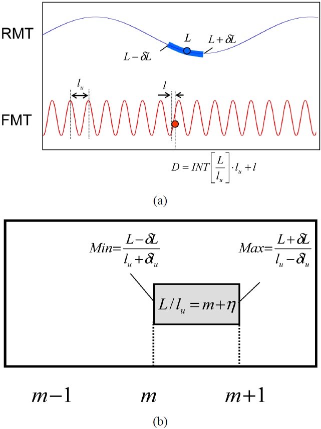
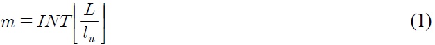
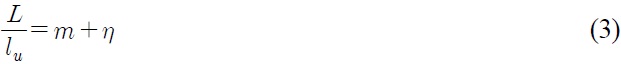
To describe the principle of combined interferometry, at least two measurement results which have well-defined unambiguity ranges, resolutions and measurement uncertainties are needed. For this discussion, a rough measurement technique (RMT) is defined as the method, which has a relatively poor resolution and a long unambiguity range. On the other hand, a fine measurement technique (FMT) is set as the method with a high resolution and its unambiguity range is small. These two techniques are simultaneously used to measure the same distance. In this case, the multiple integer order (
where

where
A typical example is the RF synthetic wavelength interferometry using the harmonics of repetition frequency (mode spacing frequency) in a femtosecond pulse laser. Assuming the repetition frequency of the femtosecond pulse laser is 75 MHz, the synthetic wavelength and the unambiguity range caused by this frequency in the Michelson type interferometers become 4.0 m and 2.0 m, respectively. The 10th harmonic of the fundamental frequency is 750 MHz, which means the synthetic wavelength and the unambiguity range become 10 times smaller than the original ones. If these two measurement results are successfully combined, the measurement resolution can be 0.056 mm
with a 2.0 m range assuming the electronic phase resolution is 0.1°. Combining these two techniques can enhance the dynamic range by a factor of 10 (in this example) while the original techniques have a dynamic range driven by the resolution of the phase meter.
The most important consideration in Eq. (2) is properly determining
The ratio (
where

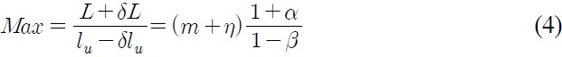
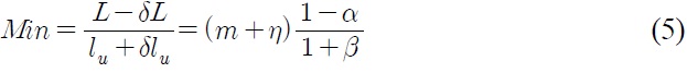
To simplify Eq. (4)-(6) further, two special cases are considered
(1) Case 1:
When the relative measurement uncertainty of the RMT (
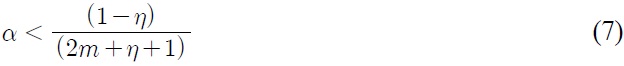

According to Eq. (7) and (8), a large
(2) Case 2:
In most of measurements, the stability of the unambiguity range is very high because of the stabilization methods, which is a more realistic representation of the actual system. (The typical wavelength stability is better than 10-9 in typical interferometer applications.) Under this assumption, the conditions from Eq. (4)-(6) are
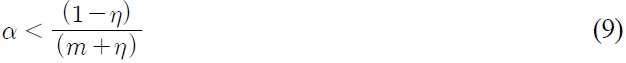

Although Eq. (9) and (10) are twice the values from Eq. (7) and (8), as was the situation in Case 1, the same criteria for Case 1 exists for Case 2. For a successful operation of the combined technique,
However, it is possible to determine

If

In the previous example, the calculated distance, 35.9135 mm is out of range based on Eq. (11) if
To summarize, the procedure for combining distance measurement techniques is as follows. First, the unambiguity range, resolution, and uncertainty for each measurement technique should be defined and the distances from each technique are measured simultaneously. Second, the multiple orders of the unambiguity range in the FMT are calculated using Eq. (1). Finally, the calculated distance is verified with Eq. (12). If the measured result fails this check, the integer should be increased or decreased by one and rechecked. For long distance measurements, the measurement uncertainty of the RMT should be enhanced according to Eq. (12).
III. EXPERIMENT AND DISCUSSION
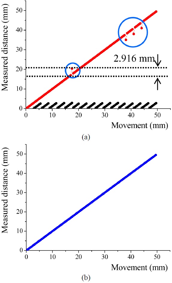
Figure 2 shows a combined technique using synthetic wavelength interferometry for the RMT and a spectrally-resolved interferometer for the FMT compared with a displacement interferometer (5510A, Agilent). The combined measurement adopted a femtosecond pulse laser as the source for both techniques simultaneously and the distance measurements had steps of 0.5 mm with a 50 mm range. The synthetic wavelength interferometer measured distances
[TABLE 1.] Calculated and compensated distances at 4 jump points (mm)
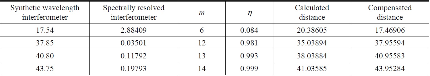
Calculated and compensated distances at 4 jump points (mm)
with the 13th harmonic of the femtosecond laser repetition frequency (75.164 MHz), which leads to an unambiguity range of 0.154 m. The phase between the reference and measurement waves was measured using a commercial lock-in amplifier (SR830, SRS). In this case, the measurement uncertainty was 0.7 mm and was mainly dominated by nonlinearity errors and phase measurement errors in the lock in amplifier. The spectrally-resolved interferometer had an unambiguity range of 1.458 mm which was determined by a solid type Fabry-Perot etalon [7].
For the first time, the measurement results in the spectrally- resolved interferometer were fixed in the form of a saw-tooth wave from the original triangular wave form [7] for simple operations as shown in Fig. 2(a) and the unambiguity range became twice the original one of 2.916 mm. The relative measurement uncertainty was 10-5 which was mainly caused by the spectrometer. As the results, it was confirmed that the condition in Eq. (12) was satisfied (0.7 mm < 1.458 mm). Fig. 2(a) also shows the combined results using Eq. (2). In the results, four points have the wrong
The first jump point is at 17.526 mm and the measurement results from the synthetic wavelength interferometer and the spectrally resolved interferometer are 17.54 mm and 2.884 mm, respectively. The integer count
On the other hand, another important issue with combining techniques is the total measurement uncertainty. From Eq. (2), the total measurement uncertainty (
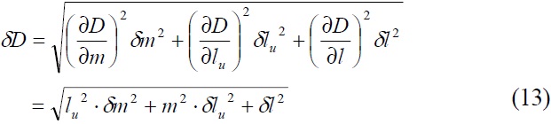
where
In this paper, we describe the principle using combined techniques to measure distances and define conditions for successful implementation of these techniques. When combining the fine measurement technique (FMT) with the rough measurement technique (RMT), the uncertainty of the RMT should be at least smaller than the half unambiguity range of the FMT. In this experiment, the synthetic wavelength interferometer and spectrally-resolved interferometer were combined to verify the techniques for the proposed conditions. Under these conditions, it was confirmed that the total measurement uncertainty can follow the measurement uncertainty of the FMT as expected.