검색 전체 메뉴
PDF
맨 위로
OA 학술지
Assessment of Gradient-based Digital Speckle Correlation Measurement Errors
  • 비영리 CC BY-NC
  • 비영리 CC BY-NC
ABSTRACT
Assessment of Gradient-based Digital Speckle Correlation Measurement Errors
KEYWORD
Gradient-based digital speckle correlation method , Measurement errors , Subset deformation mismatch
  • I. INTRODUCTION

    Digital Speckle Correlation Measurement (DSCM) is an optical technique developed for full field and non-contact measuring of surface displacement and deformation [1]. This method utilizes a natural or artificial surface speckle pattern as an information carrier and sum of squared differences or cross correlates two slightly different images captured before and after a deformation, to obtain the whole field displacement of a planar specimen surface.

    An important issue about the DCSM method is accuracy and precision. There are several factors influencing the accuracy of the DSCM method. The measurement errors may be classified in two types: errors associated with the experimental setup (acquisition system, illumination conditions) and errors associated with the correlation algorithm. The experimental errors are related basically to the variations of illumination and the quality of the acquisition system, i.e., the noise during the acquisition and digitalization [2], the camera lens distortion [3], position of the camera respect to the specimen, etc. The errors related to the algorithm are due to different choices of the implementation of the algorithm, such as the choice of the subset size [4,5], correlation function [6], sub-pixel interpolation algorithm [7,8], subset shape function [9,10] and speckle pattern quality [11]. Recently, analytical results have been derived about the effect of random image noise on the precision of displacement measurements by the DSCM method for rigid body motion estimation [12]. In [7], the performance of three most used sub-pixel algorithms were compared for simulated images. These algorithms were known as curve -fitting, gradient-based and Newton-Raphson algorithms. The results showed that the Newton-Raphson approach is the more accurate and stable. But its computation time is much longer than that of gradient-based algorithms. Taking into the requirements both in calculation accuracy and in calculation speed, the gradient-based method is a better replacement of the Newton-Raphson method. Other interesting approaches like the use of genetic algorithms, finite elements and B-splines are reported in [13], but it appears to have a lower performance than gradient-based algorithms in terms of accuracy. A study of the systematic errors due to use of shape functions of lower order than the actual displacement field was presented in [9]. Some requirements were presented about properties of the pattern, subset size and order of the shape functions. In [4], a theoretical model of the displacement measurement accuracy of DSCM was accurately predicted based on the variance of image noise and Sum of Square of Subset Intensity Gradients (SSSIG). The model further led to a simple criterion for choosing a proper subset size for the DSCM analysis. Further, in [11], it proposed the Mean Intensity Gradient to obtain the optimal subset size, where the Newton -Raphson algorithm was used, the simplest correlation coefficient and the zero-order shape function for pure in-plane translation tests. In [14], a method was presented to estimate an appropriate pattern density for different subset sizes determining the characteristic sampling length of the speckle granules. From the above descriptions, it can be seen that assessment of DSCM measurement errors in practice is important but confusing. The measurement accuracy of DSCM depends on a number of factors. The effects of these factors (e.g. speckle pattern, out of plane displacement, lens distortion, noise, subset size, sub-pixel registration algorithm, shape function, interpolation scheme) have been investigated separately in previous studies. Few reported quantitative works have been performed to systematically evaluate the gradient-based DSCM measurement errors. Therefore, understanding the major constituent of gradient-based digital speckle correlation measurement errors and describe them in mathematical derivation is necessary and helpful.

    In this study, an analysis has been carried out on the standard deviation of displacement measurement errors by gradient-based DSCM. A new formulation will be used to explicitly account for the image grayscale error due to sub-pixel interpolation errors, image noise, and subset deformation mismatch at each point of the subset. Numerical and experiment results of error estimation will be presented to validate the analytical formulas on the standard deviation of displacement measurement errors, and to assess individual and combined effects of sub-pixel interpolation errors, image noise, and subset deformation mismatch on the precision of displacement measurements. The final formulation can not only be used to predict the displacement measurement error, but also to give us some hints on how to improve the displacement measurement precision of DSCM.

    II. FUNDAMENTAL PRINCIPLE OF GRADIENT-BASED DSCM

    The DSCM involves recording, digitizing and processing a pair of speckle patterns of an object in different deformation states, one before deformation and the other after deformation. The DSCM process is generally divided into two different stages. The first stage takes discrete, one pixel steps and correlates each one. The highest correlation is then taken to be the starting point for the next stage, which uses interpolation for sub-pixel accuracy. In routine practice of the DSCM method, a cross-correlation criterion or sum -squared-difference correlation criterion is predefined to evaluate the similarity between the reference image subset and the current image subset. The sub-pixel registration algorithm is considered as a key technique to improve displacement measurement accuracy in DSCM [7]. There are multiple ways to achieve sub-pixel accuracy that have been used successfully.

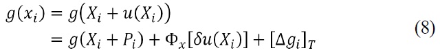
    The gradient-based method as one of the DSCM methods is introduced to measure sub-pixel displacement because of its high efficiency and precision [15,16]. This method was originally developed by Davis and Freeman for use in video compression and is based on first-order spatio-temporal gradients. It starts with an assumption that the image misalignment is purely translational. This assumption is deemed to be reasonable when the subsets are small. For simplicity, both grayscale intensity value of pixels in the deformation direction of reference image G(X) before deformation and its corresponding current image g(x) after deformation will be given as a single row matrix [17]. The corresponding subset s in the current image g(x) is related to the subset S in the reference image G(X) by a so-called subset shape function u(X) via x = X + u(X), which is utilized to approximate the underlying deformation field. With gray level conservation assumption it can be assumed that the relationship in Equation (1) holds true.

    image

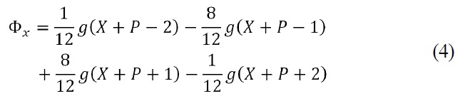
    A zero-order shape function is employed due to the pure in-plane rigid body translation of the subset, it has

    image

    where p1 is the whole-pixel translational displacement, and p2 is the corresponding sub-pixel displacement in the deformation direction. The pixel points in the reference image subset S = [X1, ···, X2] all have integral pixel coordinates, so Xi is always integral-valued. However, the corresponding pixel points in the current image subset s = [x1, ···, x2] are generally non-integral pixel coordinates, so xi is usually real-valued.

    Let us assume that the integer pixel portion of the displacement (P) is known. The unknown displacement field is sought in the form u(X) = P + δu(X), where the displacement correction δu(X) is assumed to be small enough to allow for a first-order Taylor expansion. So, the grayscale intensity value of the current image g(x) at non-integral pixel locations may be approximated by a Taylor expansion around the whole-pixel locations of the current image

    image

    where the term P = int(p1 + p2) is the integer pixel portion of the displacement, [Δgi]T are higher order terms of the Taylor expansion, δu(X) = u(X) - P is non-integral pixel portion of the displacement. Φx is the first-order derivatives of grayscale intensities at point X + P of the current image. It can be calculated by the convolution of the grey with the mask of [1/12, -8/12, 0, 8/12, -1/12](The mask is deduced through cubic spline interpolation of five neighboring pixels). Using this method, an approximation of the partial derivatives value at point X + P can be calculated as follow [16]

    image

    The following sum-squared-difference (SSD) correlation coefficient is introduced for deriving a theoretical model of the displacement measurement accuracy of DSCM. The SSD correlation function is defined as

    image

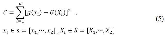
    Minimization of the SSD correlation coefficient would provide the best estimate of the desired displacements. Thus we have

    image

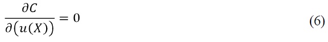
    The iterative solution methods such as the Newton -Raphson method or Levenberg-Marquardt method can be used to solve the above nonlinear equation.

    III. ERROR EVALUATION OF GRADIENT-BASED DSCM

    It is noted that the displacement measurement accuracy

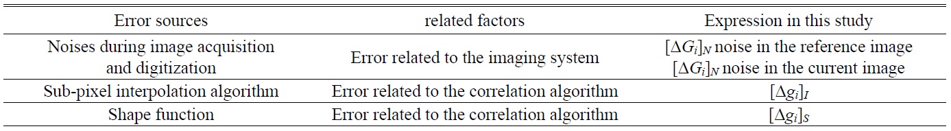
    [TABLE 1.] Error sources of gradient-based DSCM and their expression

    label

    Error sources of gradient-based DSCM and their expression

    of DSCM relies heavily on the perfection of the imaging system and the selection of a particular correlation algorithm. The errors discussed in this study are given in Table 1.

    The image noise defined here will consist of both random white noise and quantization error in each image. If noise [ΔGi]N in the reference image and noise [ΔGi]N in the current image can be fully accounted for, there would be a perfect match between the corrected reference image G(Xi)-[ΔGi]N , and the corrected current image g(xi)-[ΔGi]N , namely,

    image

    The grayscale level of the current image g(xi) at non -integral pixel locations may be approximated by a Taylor expansion around the whole-pixel location Xi + Pi of the current image

    image

    where δu(Xi) = u(Xi)-Pi. Equation (8) is the same as Equation (3). If the subset deformation is approximated by the zeroorder shape function as given in Equation (2), one has

    image

    where [Δgi]S is the error due to the approximate subset shape function used. If the gradient Φx is to be approximated by cubic spline interpolation in Equation (4), one has,

    image

    where δΦx is the cubic spline interpolation error, Equation (10) can be rewritten as

    image

    where [Δgi]I =δΦx [p1 + p2-Pi] + [Δgi]T is the interpolation error for approximating the current image g(xi) at non-integral pixel locations. By combining Equation (7) and (11), one has

    image

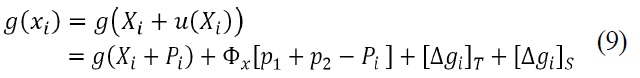
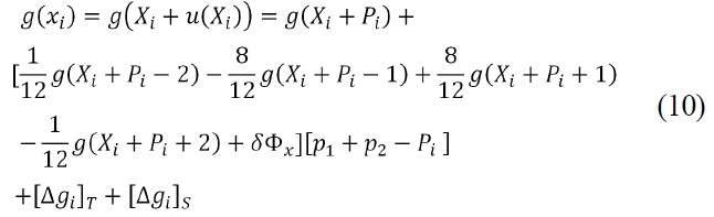
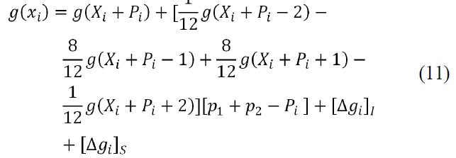
    In practical applications, some ideal situation such as (1) both reference image and current image are noise-free; (2) the subset deformation can be accurately described by the a zero-order shape function; may not be met. So under non-ideal situations, the deformation parameters p1 and p2 will be displaced by p1 + Δp1 and p2 + Δp2 respectively, where Δp1 and Δp2 are the error in the estimated wholepixel displacement and sub-pixel displacement due to the existence of image noise and shape function approximation. The zero-order shape function can be written as

    image

    The minimization of the SSD correlation coefficient
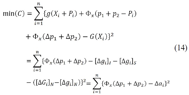
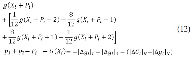
 C in Equation (5) can then be expressed as

    image

    Term Δai = [Δgi]I + [Δgi]S + [ΔGi]N - [Δgi]N

    represents a sum grayscale errors at each pixel point and its existence usually results in the non-zero errors Δp1 and Δp2. That means, when the image grayscale error at each pixel point Δai = 0, one would have Δp1 = 0 and Δp2 = 0, namely, Δp = 0.

    If both p1 and p2 are known, the image grayscale error Δai at each point of the subset can actually be computed from

    image

    So displacement error Δp (contains both the error of whole-pixel and sub-pixel displacements) can be computed from

    image

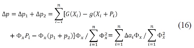
    As shown in the analyses above, the deformation errors in DSCM are unavoidably. It is assumed that the image grayscale error Δ
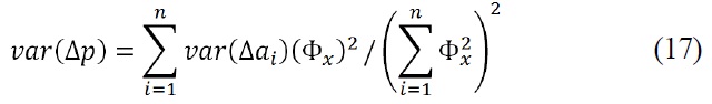
ai at each point maintains a statistically random character and has a Gaussian distribution with a zero mean. The variance of displacement errors are given as

    image

    If varai) is the same for every point, varai) = vara), Equation (17) can be further simplify as the following

    image

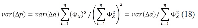
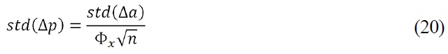
    Furthermore, the standard deviation errors of the displacement measurement can be expressed as

    image

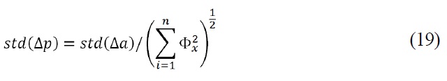
    It is evident from Equation (18) and (19) that the displacement accuracy of DSCM is determined by the image grayscale error Δa (consisting of sub-pixel interpolation error ([Δgi]I), image noise ([ΔGi]N, [Δgi]N), and the mismatch between the assumed subset shape function and the actual deformation field of the subset ([Δgi]S)) and first-order derivatives of grayscale intensities Φx.

    In addition, if Φx is a nearly constant contrast at every point in the subset, then the standard deviation errors from Equation (19) can be rewrite as

    image

    IV. RESULTS OF NUMERICAL SIMULATIONS

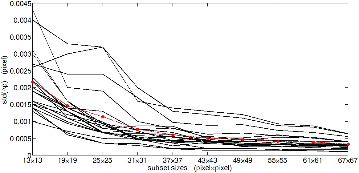
       4.1. Effects of Sub-pixel Interpolation When the reference and current image are

    When the reference and current image are free of random white noise ([ΔGi]N = 0, [Δgi]N = 0) and the zero-order subset shape function matches the actual deformation field ([Δgi]S = 0), the sub-pixel interpolation error [Δgi]I will be the main factor affecting the accuracy and precision of deformation estimation. Fig. 1 shows a summary of the standard deviation in displacement estimation error stdp)

    over a range of subset sizes for 20 image pairs with 20 different rigid body translations (p1 + p2 = 0.005, 0.007, 0.016, 0.024, 0.038, 0.041, 0.053, 0.069, 0.077, 0.082, 0.15, 0.78, 1.01, 1.40, 1.62, 1.81, 1.96, 2.39, 2.74, 3.18 pixels).

    While stdp) is found to decrease with increasing subset size, The standard variation of the average values of stdp) of all 20 image pairs with the subset size (total n pixels) are also shown in Fig. 1 as a dashed line with discrete symbols for each data point. The dashed line is a power-law curve fitting of the discrete data points in the form of stdp) = anb with a = 0.04046 and b = -0.5683 (SSE: 2.1e-8, R-square: 0.9935). The exponent b is close to -0.5 (see Equation 20), indicating that the image grayscale error does following the assumption made previously in deriving Equation (20). In addition, the actual value of average standard deviation due to sub-pixel interpolation error is rather small: stdp) = 0.000511 pixels at subset size n = 43.

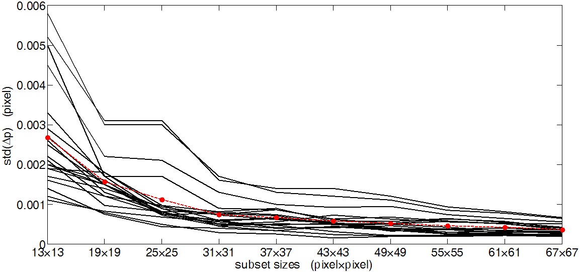
       4.2. Effects of Random White Noise

    Add Gaussian noise of 0 mean and variance (σ2) of 0.2 pixels to the reference and current image. Fig. 2 shows the effect of random white noise on the standard deviation in displacement estimation error stdp) over a range of subset sizes for 20 image pairs with 20 different rigid body translations (p1 + p2 = 0.005, 0.007, 0.016, 0.024, 0.038, 0.041, 0.053, 0.069, 0.077, 0.082, 0.15, 0.78, 1.01, 1.40, 1.62, 1.81, 1.96, 2.39, 2.74, 3.18 pixels). The dashed line is a power-law curve fitting of the discrete data point in the form of stdp) = anb with a = 0.07484 and b = -0.6617 respectively (SSE: 2.96e-8, R-square: 0.9937). Again the stdp) decrease in general with increasing subset sizes for all image pairs. But the exponent b is deviate slightly from -0.5. On average, the actual value of average standard deviation due to sub-pixel interpolation error and random white noise is still small: stdp) = 0.0005823 pixels at subset size n = 43, somewhat larger than the former case in above section.

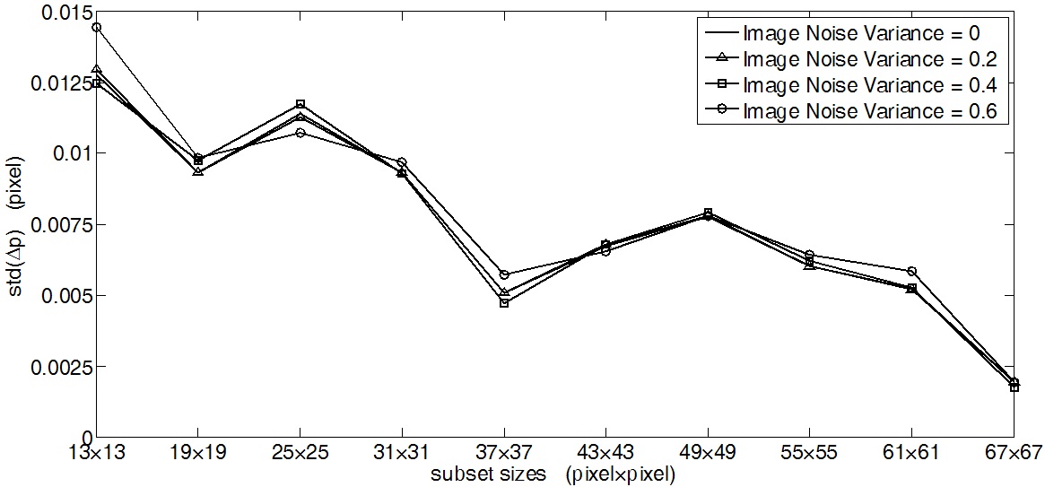
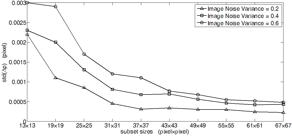
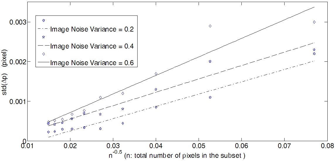
    Figure 3 shows the effect of different random white noise levels (σ2 = 0.2, 0.4 and 0.6) on the standard deviation

    in displacement estimation error stdp) over a range of subset sizes for an image pair with a rigid body translation only (p1 + p2 = 0.041). The standard deviation in displacement estimation error decreases with the increasing random white noise variance. Fig. 4 using n(-0.5) as the horizontal-axis coordinate instead of n. A nearly linear dependence of stdp) on n(-0.5) seems to exist (stdp) =an(-0.5) + b); dash-dotted line, dashed line and solid line represent the linear fitting on the displacement estimation error stdp) of n(-0.5) under different image noise levels. Specifically, the actual values of a and b are 0.03102 and -3.6780e-4 (with SSE:

    1.595e-7, R-square: 0.9544), 0.03379 and -1.246e-4 (with SSE: 1.995e-7, R-square: 0.952), 0.04676 and -2.181e-4 (with SSE: 6.128e-7, R-square: 0.9252) respectively for three different image noise levels.

       4.3. Effects of Subset Shape Function Mismatch

    The analysis above does not consider the mismatch of shape function. In practice, the deformations may contain the displacement gradient ε, which means that the deformations of subset are no longer pure rigid body translation. Fig. 5 shows the effect of displacement gradient (ε = 0.002, p1 + p2 = 0.041) on the standard deviations of displacement estimation error stdp) under different image noise levels. Four image pairs with different random image noise levels (σ2 = 0, 0.2, 0.4 and 0.6) are shown in the figure. Clearly, the power-law relationship observed previously for stdp) no longer holds and the values of stdp) are significantly increased. The diversity of variance in different noise levels is no longer a key factor affecting the displacement estimation error. In fact, stdp) is found not to decrease monotonically with increasing subset sizes. The obvious fluctuation of these curves reflects the detrimental effect of major subset shape function mismatch [Δgi]S when the order of the assumed subset shape function was lower than that of the actual subset shape field.

    V. RESULTS OF EXPERIMENT

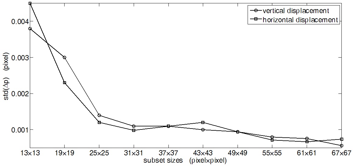
       5.1. The Self-correlation Experiment

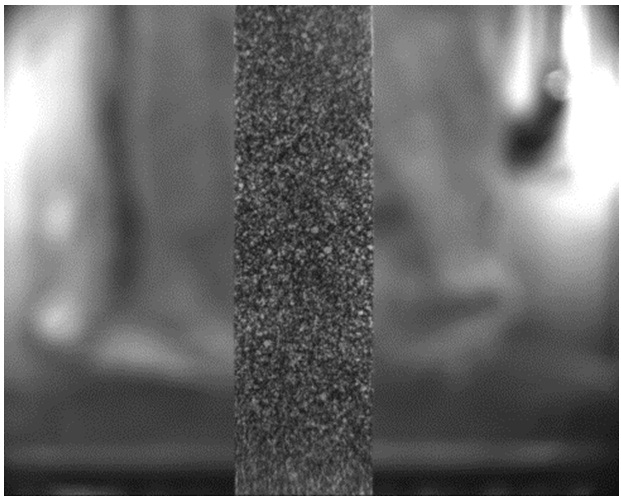
    The self-correlation experiment is proposed by Z.Y. Wang et al [12]. It acquires two images by CMOS without moving the object. The first image is denoted by α, and the second image is denoted by β , α and β are not identical due to noise. Then they calculate the displacement fields between α and β by DSCM. The difference between α and β is denoted by γ, γ =α -β. The elements of γ are noise values of different pixels. By using this method, we can analyze the effect of noise γ on the displacement estimation errors. As stated before, the acquired image α is shown in Fig. 6. The image β is not presented because it

    is very similar to α. The images are obtained by a CMOS-based digital image acquiring system, which permits recording of images with a size of 1280×1024 pixels with 256 gray levels each. The random speckle pattern in the images is created by lightly spraying some white and black paint on the specimen. The specimen is illuminated by ordinary white light.

    Figure 7 is the results concerning both the vertical and horizontal displacement estimation errors, it shows that the displacement estimation error decreases when subset size increases. For different directions, the power-law relationship observed roughly for stdp) in the form of stdp) = anb, Specifically, the actual values of a and b are 0.07034 and -0.5673 (with SSE: 5.765e-7, R-square: 0.9441), 0.1646 and -0.7099 (with SSE: 8.429e-7, R-square: 0.932) respectively for the vertical and horizontal directions.

       5.2. Rigid Body Translation

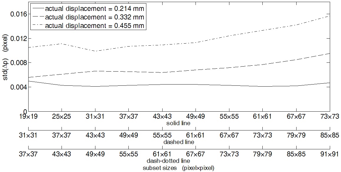
    In this section, the specimen is the same as the one used in the self-correlation experiment. The sample is attached to the universal material experimental machine with a translation accuracy of 2 μm. Three images of the speckle pattern with a given vertical direction rigid body translation (0.214 mm, 0.332 mm and 0.455 mm respectively) are captured by the same CMOS-based digital image acquiring system.

    The mean displacement of the rigid body translation calculated by DSCM is 16.2653 pixels, 25.3415 pixels and 34.9853 pixels, respectively. Clearly, there is a linear relationship between actual displacements (Uact) in millimeters

    and calculated displacements (Ucal) in pixels, it can be expressed in the form of Ucal = aUact + b with a = 0.01287 and b = 0.005018 respectively (SSE: 8.87e-7, R-square: 1), the coefficient a is the conversion factor between actual displacements and calculated displacements, which means each pixel represents 12.87 μm.

    Figure 8 shows the standard deviations of displacement estimation error stdp) of different actual displacements. In fact, contrary to Equation (20), stdp) is found to increase rather than decrease with increasing subset sizes. Furthermore, stdp) increase with increasing actual displacements for these three image pairs. The most probable reason for the increasing trend in stdp) with increasing subset sizes is that the displacement (in pixels) violates one of gradient -based DSCM assumptions, the displacements of subsets are small. The underlying deformation field of a small subset can be readily and accurately approximated by a zero-order subset shape function, whereas a larger subset size normally leads to larger errors in the approximation of the underlying deformations [4]. For this reason, to guarantee a reliable displacement measurement, a small subset size is preferable in this section. This problem can be avoided by increasing the distance between the lens and the specimen. It means that each pixel of current image represents a large displacement (in millimeters).

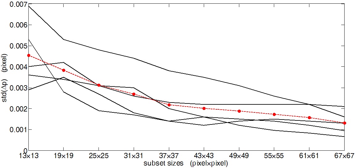
    Rigid body translation experiment was re-run. The sample is attached to the universal material experimental machine. Five images of the speckle pattern with a given vertical direction rigid body translation (0.008 mm, 0.015 mm, 0.023 mm, 0.030 mm and 0.035 mm respectively) are captured by the CMOS-based digital image acquiring system. Fig. 9 shows a summary of the standard deviation in displacement estimation error stdp) over a range of subset sizes for 5 image pairs with 5 different rigid body translations mentioned above.

    The power-law relationship observed roughly for the average values of stdp) (dashed line with discrete symbols) in the form of stdp) = anb, Specifically, the actual values of a and b are 0.02846 and -0.3499 (with SSE: 1.573e-7, R-square: 0.9842).

       5.3. Three-point Bending

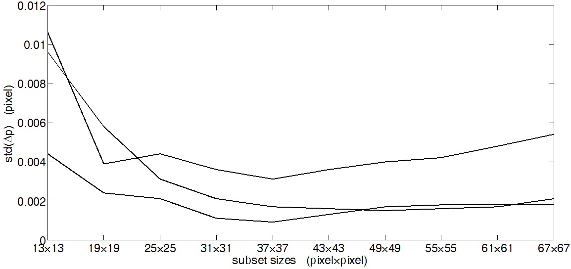
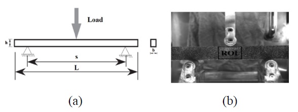
    In this section, a three-point bending test of a steel specimen was carried out. The dimensions of the three-point bending specimen are shown in Fig. 10. The experimental device was a universal material experimental machine. First, the specimen was recorded before loaded as the reference image. Then a load P was applied to the specimen. With the load increased, images of the Region of Interests (ROI) was captured at P = 4333.73N, 8659.89N and 12851.17N. These images were analyzed using the DSCM. Fig. 11 shows a summary of the standard deviation in displacement estimation error stdp) of the center point of ROI over a range of subset sizes for 3 image pairs with 3 different load conditions.

    The power-law relationship observed previously for std (Δp) no longer holds. In fact, stdp) is found not to decrease monotonically with increasing subset sizes for all image pairs and the subset size that has a minimum value of stdp) is usually between 31×31 to 37×37 pixels. The increasing trend in stdp) with increasing subset sizes at large subset sizes (say n > 43 pixels) reflects the detrimental effect of major subset shape function mismatch [Δgi]S when the order of the assumed subset shape function (zero-order) was lower than that of the actual subset deformation field.

    VI. DISCUSSION

    Deformation estimation errors by DSCM have been reformulated with an explicit representation of the image grayscale error Δai at each point of a subset. Sub-pixel interpolation error ([Δgi]I), image noise ([ΔGi]N, [Δgi]N) and the mismatch between the assumed subset shape function and the actual deformation field of the subset ([Δgi]S) have been identified as major sources of grayscale errors that affect the accuracy and precision of deformation measurement.

    The sub-pixel interpolation error and image noise error would always be present and they can be affected by the actual image intensity profile characteristics and deformation field characteristics [12]. Nevertheless, the image grayscale error due to sub-pixel interpolation and image noise in the simulated image pairs analyzed in this study were relatively small (the average values of stdp) even at a small subset size of 43 × 43 pixels were no more than 0.0005 pixels and 0.0006 pixels respectively). Similarly, the effect of sub-pixel interpolation and image noise in the self -correlation experiment and rigid body translation experiment were still small (the average values of stdp) even at a small subset size of 43 × 43 pixels were no more than 0.0012 pixels and 0.0022 pixels respectively; they were about 3 to 4 times larger than the simulated image pairs). Values of stdp) at subset size 43 × 43 pixels were about 0.00076 pixels when the random white noise variance was σ2 = 0.6 and the displacement was 0.041 pixels. It was about 1.4 times of in images with zero random white noise at the same subset size. Variance of displacement errors stdp) increased significantly due to the combined effect of sub-pixel interpolation, image random noise and their dependence on the subset size followed a power-law relationship with their exponents around -0.3499 and -0.7077. Finally, there was an even more significant effect due to the third type of errors [Δgi]S) when the zero-order subset shape function was used for an image pair deformed with a non-zero displacement gradient. Whether numerical simulation, or three-point bending test, not only the power -law dependence on the subset size broke down, but the resulting errors were also much higher (see Fig. 5 and Fig. 11).

    Several assumptions were made to obtain the power-law relationships on the variances of displacement errors. Those assumptions might not all strictly apply to any real experimental conditions, even numerical simulation. Pan et al. extended the error analysis of two-dimensional motion estimation [4] to include detailed analyses on bias in displacement estimation when random white noise existed in both reference and current images. Their results showed the bias in displacement measurements depends on both the variance of image noise and Sum of Square of Subset Intensity Gradients (SSSIG). But the effect of possible subset shape mismatch was not considered by them. If the image noise ([ΔGi]N, [Δgi]N) consisting of random white noise with a zero mean and a variance of σ2 dominates the image grayscale error Δaiai = [ΔGi]N - [Δgi]N), Equation (19) can be rewritten as follow

    image

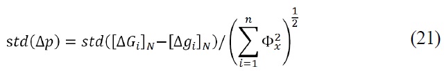
    Equation (21) becomes identical to Equation (18) and (19) given by Pan et al. in [4]. Similarly, Equation (21) provides a criterion for subset size selection in DSCM. For certain CMOS-based digital image acquiring system, the image noise can be accurately quantified by self-correlation experiment mentioned above. The displacement measurement accuracy can be controlled by adjusting the value of SSSIG [4], which can be increased or decreased by adjusting the subset size. Furthermore, Equation (20) leads to a simple criterion for choosing a suitable subset size, image quality, sub-pixel algorithm, and subset shape function for DSCM for the desired measurement precision.

    VII. SUMMARY

    Deformation measurement errors of gradient-based DSCM analysis have been presented in terms of sub-pixel interpolation error, image noise, and subset deformation mismatch. A new formulation is used to explicitly account for the image grayscale error due to above three error sources at each point of the subset. Numerical and experiment results of error estimation are presented to validate the analytical formulas on the standard deviation of displacement measurement errors. It has been shown that 1) Deformation measurement errors are directly linked to the image grayscale error at each point of the subset; 2) The standard deviation of displacement measurement errors stdp) on the subset size is actually a power-law relationship with an exponent of -0.3499 and -0.7077 when the sub-pixel interpolation error and image noise are dominant of the image grayscale error. The power-law relationship further leads to a simple criterion for choosing a suitable subset size, image quality, sub-pixel algorithm, and subset shape function for DSCM; 3) When the power-law dependence clearly breaks down, the subset deformation mismatch may become dominant and there is an upper limit of the subset size for minimizing errors.

참고문헌
  • 1. Sutton M. A., Turner J. L., Bruck H. A., Chae T. A. (1991) “Full-field representation of discretely sampled surface deformation for displacement and strain analysis” [Express Mech.] Vol.31 P.168-177 google
  • 2. Smith B. W., Li M., Tong W. (1998) “Error assessment for strain mapping by digital image correlation” [Express Tech.] Vol.22 P.19-21 google
  • 3. Bing P., Xie H.-m., Chen P.-w., Huang F.-l., Zhang Q.-m. (2009) “Assessment and correction of lens distortion for digital image correlation” [Acta Metrologica Sinica] Vol.30 P.62-67 google
  • 4. Pan B., Xie H., Wang Z., Qian K., Wang Z. (2008) “Study on subset size selection in digital image correlation for speckle patterns” [Opt. Express] Vol.16 P.7037-7048 google cross ref
  • 5. Lecompte D., Smits A., Bossuyt S., Sol H., Vantomme J., Van Hemelrijck D., Habraken A. M. (2006) “Quality assessment of speckle patterns for digital image correlation” [Optics and Lasers in Engineering] Vol.44 P.1132-1145 google cross ref
  • 6. Wang H., Kang Y., Heping X. (2005) “Advance in digital speckle correlation method and its application” [Advance in Mechanics] Vol.35 P.195-203 google
  • 7. Pan B., Xie H.-m., Xu B.-q., Dai F.-l. (2006) “Performance of sub-pixel registration algorithms in digital image correlation” [Measurement Science and Technology] Vol.17 P.1615-1620 google cross ref
  • 8. Schreier H. W., Braasch J. R., Sutton M. A. (2000) “Systematic errors in digital image correlation caused by gray-value interpolation” [Opt. Eng.] Vol.42 P.2915-2921 google
  • 9. Shreier H. W., Sutton M. A. (2002) “Systematic errors in digital image correlation due to under matched subset shape functions” [Express Mech.] Vol.42 P.303-310 google
  • 10. Lu H., Cary P. D. (2000) “Deformation measurements by digital image correlation: implementation of a second-order displacement gradient” [Express Mech.] Vol.40 P.394-400 google
  • 11. Pan B., Lu Z., Xie H. (2010) “Mean intensity gradient: an effective global parameter for quality assessment of the speckle patterns used in digital image correlation” [Optics and Lasers in Engineering] Vol.48 P.469-477 google cross ref
  • 12. Wang Z. Y., Li H. Q., Tong J. W., Ruan J. T. (2007) “Statistical analysis of the effect of intensity pattern noise on the displacement measurement precision of digital image correlation using self-correlated images” [Express Mech.] Vol.47 P.701-707 google
  • 13. Pan B., Qian K., Xie H., Asundi, A. (2009) “Two-dimensional digital image correlation for in plane displacement and strain measurement: a review” [Measurement Science and Technology] Vol.20 P.062001 google cross ref
  • 14. Sutton M. A., Orteu J. J., Schreier H. W. 2009 Image Correlation for Shape, Motion and Deformation Measurements: Basic Concepts, Theory and Applications google
  • 15. Davis C. Q., Freeman D. M (1998) “Statistics of subpixel registration algorithms based on spatiotemporal gradients or block matching” [Opt. Eng.] Vol.37 P.1290-1298 google cross ref
  • 16. Pan B., Xu B.-q., Xie H.-m. (2005) “In-plane displacement measurement by gradient-based digital image correlation” [Optical Technique] Vol.31 P.643-647 google
  • 17. Tong W., Yao H., Xuan Y. (2011) “An improved error evaluation in one-dimensional deformation measurements by linear digital image correlation” [Express Mech.] Vol.51 P.1019-1031 google
OAK XML 통계
이미지 / 테이블
  • [ TABLE 1. ]  Error sources of gradient-based DSCM and their expression
    Error sources of gradient-based DSCM and their expression
  • [ FIG. 1. ]  Summary of the standard deviation in displacement estimation error std (Δp) over a range of subset sizes for 20 image pairs with 20 different rigid body translations.
    Summary of the standard deviation in displacement estimation error std (Δp) over a range of subset sizes for 20 image pairs with 20 different rigid body translations.
  • [ FIG. 2. ]  Effect of random white noise σ2 = 0.2 on the standard deviation in displacement estimation error std (Δp) over a range of subset sizes for 20 image pairs with 20 different rigid body translations.
    Effect of random white noise σ2 = 0.2 on the standard deviation in displacement estimation error std (Δp) over a range of subset sizes for 20 image pairs with 20 different rigid body translations.
  • [ FIG. 3. ]  Effect of different random white noise levels (σ2 = 0.2, 0.4 and 0.6) on the standard deviation in displacement estimation error std (Δp) over a range of subset sizes for an image pair with a rigid body translation only (p1 + p2 = 0.041).
    Effect of different random white noise levels (σ2 = 0.2, 0.4 and 0.6) on the standard deviation in displacement estimation error std (Δp) over a range of subset sizes for an image pair with a rigid body translation only (p1 + p2 = 0.041).
  • [ FIG. 4. ]  Power-law fittings of the same results in FIG. 3.
    Power-law fittings of the same results in FIG. 3.
  • [ FIG. 5. ]  Effect of displacement gradient (ε = 0.002, p1 + p2 = 0.041) on the standard deviations of displacement estimation error std (Δp) under different image noise levels.
    Effect of displacement gradient (ε = 0.002, p1 + p2 = 0.041) on the standard deviations of displacement estimation error std (Δp) under different image noise levels.
  • [ FIG. 6. ]  Image α used self-correlation experiment.
    Image α used self-correlation experiment.
  • [ FIG. 7. ]  Both the vertical and horizontal displacement estimation errors.
    Both the vertical and horizontal displacement estimation errors.
  • [ FIG. 8. ]  Standard deviations of displacement estimation error std (Δp) of different actual displacements.
    Standard deviations of displacement estimation error std (Δp) of different actual displacements.
  • [ FIG. 9. ]  Summary of the standard deviation in displacement estimation error std (Δp) over a range of subset sizes for 5 image pairs with 5 different rigid body translations.
    Summary of the standard deviation in displacement estimation error std (Δp) over a range of subset sizes for 5 image pairs with 5 different rigid body translations.
  • [ FIG. 10. ]  (a) Dimensions of the specimen (where L = 350 mm, s = 120 mm, h = 30 mm, and b = 15 mm), (b) Region of Interests on the three-point bending steel specimen.
    (a) Dimensions of the specimen (where L = 350 mm, s = 120 mm, h = 30 mm, and b = 15 mm), (b) Region of Interests on the three-point bending steel specimen.
  • [ FIG. 11. ]  Summary of the standard deviation in displacement estimation error std (Δp) of the center point of ROI over a range of subset sizes for 3 image pairs with 3 different load conditions.
    Summary of the standard deviation in displacement estimation error std (Δp) of the center point of ROI over a range of subset sizes for 3 image pairs with 3 different load conditions.
(우)06579 서울시 서초구 반포대로 201(반포동)
Tel. 02-537-6389 | Fax. 02-590-0571 | 문의 : oak2014@korea.kr
Copyright(c) National Library of Korea. All rights reserved.