For the last decade, the performance of a single microprocessor has become as powerful as a vector computer of the previous generation. Thus, the parallel computing based on the cluster of a microprocessor system such as workstations or personal computer (PC) has become the mainstream of high-performance computing replacing vector computing. However, the change of processor architecture necessitates a new programming paradigm in addition to the vectorization or the parallelization in high-performance computing areas including computational fluid dynamics (CFD), where a large memory capacity, a lot of access to the memory devices and a huge number of computational operations are necessary.
Two of the major changes in the latest microprocessors are super-scalar architecture and memory hierarchy employing a large amount of high-speed data caches. Thus, the utilization of these two factors is the key point of maximizing the processor capability, which can be achieved by programming approaches such as the blocking method [1]. However, the blocking method is quite complex and difficult for general use and existing codes should be rewritten completely, even with the use of BLAS (Basic Linear Algebra Subprogram) a functional library for the blocking method [1,2].
In the present paper an introduction to the latest microprocessor systems and the concept of acceleration will be given first, and the way of optimizing a computational code, called here as ‘localization’, is described for a compressible fluid dynamics code using the LU-SGS (lowerupper symmetric Gauss-Seidel) solution algorithm [3]. The LU-SGS algorithm is considered since it is one of the simplest and most efficient quasi-implicit iterative matrix solution algorithms widely used these days. The localization technique has been suggested by Choi et al. to maximize the code performance without an additional subprogram, but by minor changes in the iterative solution algorithm [4]. It has been tested for Pentium III and 4 processors previously, but has been tested to confirm the effectiveness for modern processor architectures having significant advances during the last decade. The localization is applied at several levels, and the performance gains at each level are tested for several of the latest microprocessor systems generally used nowadays.
2. Processor Architecture and Memory Hier archy
From the last decades, Moore’s law, the doubling of transistors every couple of years, has governed the performance increase of micro-processors [5]. The typical circuit width in the microprocessors becomes less than 100nm and it is thought that they will face a limitation in the near future in comparison with the size of molecules. However, the current pace of the performance increase is expected to continue for the time being based on the development of the circuit design technology and the manufacturing technology, such as photolithography. The number of transistors was around 3 million in the Pentium® processor, but becomes greater than 40 million in the Pentium® 4 Processors, and currently stands at 1.5billion. Owing to such a tremendous integrity, a super-scalar architecture, such as the pipelines and the vector processing used in supercomputers previously, can be embodied in a single microprocessor to handle several instructions at a time. In addition, the operating speed of the newest microprocessor becomes greater than 3GHz, which implies that GFlops (Giga-floating-point operations per second), which was only possible with a supercomputer, would be feasible with a single processor [6-9].
Meanwhile, the peripheral devices, including system’s main memory are developed further not only for the capacity but also for the operating speed and the data bandwidth. SDRAM (synchronous dynamic random-access memory), RDRAM (Rambus dynamic random-access memory) and DDR SDRAM (Double Data Rate Synchronous Dynamic Random-Access Memory) are examples of the high-speed memory devices employed in the latest computer systems. However, the data processing speed of the memory devices is still slower than the internal processing speed
of microprocessors, and the time consumed during the communication with the system’s main memory and other external devices take a large portion of overall computational time, rather than the computation itself.
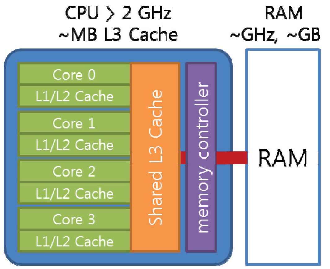
Therefore, a cache, a high-speed temporary storage device for the frequently used data and instructions, has been employed to fill the gap between the main memory and the microprocessor, since the development of 32 bit microprocessors. The cache has been employed in two levels. The first level (L1) cache was included inside the microprocessor for the frequently used instructions, and a small amount of data used most often. The second level (L2) cache has been employed outside the microprocessor for the large amount of frequently used data using the highspeed memory device, such as SRAM (static random-access memory). The Pentium processor had the L2 cache outside the processor, but further performance improvement was limited since the cache performance was limited by the speed limit of the system’s data bus (called as front-sidebus, FSB) connecting the processor and other peripherals. The Pentium II processors employed an independent cache bus (called as back-side-bus, BSB) that can be operated at the half speed of the processor. Fig. 1 shows the schematics of the data bus architectures for modern microprocessors. After the Pentium III processors, on-die L2 cache, which operates at the same speed of the processor, is included in many of the microprocessors, such as Intel Pentium 4, AMD Athlon processors. The Pentium 4 Processor operating at 1.7GHz having the data transfer rate to the system’s main memory is limited to 3.2 GB/s using RDRAM and to 1.03 GB/s using SDRAM. However, the data transfer rate between the processor and L2 cache is 54 GB/s, which is 17 to 50 times faster than the main memory [10,11]. Thus, the third-level cache is considered for next-generation systems though not common yet. These characteristics of the memory hierarchy are quite common to many of the latest microprocessor systems though their architectures are different. The amount of L2 caches ranges from 64KB to 4MB, but 128, 256 or 512 KB on-die L2 cache is common these days. The amount of 256 KB is equivalent to 32,768 8Byte (64bit or 32 bit double precision) real variables, which is equivalent to 3,276 computing nodes having 10 variables per node. Thus, the utilization of the high-speed L2 cache has the key-role for the performance of the computational codes.
3. Acceleration of Computing Codes
The way of accelerating the computational codes can be classified in two categories: 1) active utilization of super-scalar architectures and 2) efficient utilization of memory hierarchy. Super-scalar is computer processor architecture that can execute multiple operations at a time. Pipelining and vector processing are the examples of super-scalar architectures previously used for vectortype supercomputers. Multiple data can be processed simultaneously and sequentially without interruption through a number of pipelines. A tremendous number of transistors needed for the super-scalar architectures can be integrated within a single microprocessor nowadays owing to the modern semiconductor integration technologies. The super-scalar architecture is embodied as several different technologies depending on the systems such as SSE2 (Streaming SIMD (Single instruction multiple data) Extension 2) for Intel Pentium 4, 3DNow! for AMD Athlon and Velocity Engine for Apple Macintosh.
The utilization of these technical characteristics means the optimization of data control within the loops of the code. However, it is not only difficult to compose a code optimized for specific machine architecture with a high-level language such as Fortran, but also not so meaningful to compose an optimized code for a specific architecture considering the continuously changing computing environment. Thus, the utilization of super-scalar architecture is limited to maintaining the general characteristics of vector processing when developing a computing code using a high-level language, and it is desirable to use compilers that can produce an optimized execution code for specific machine architecture. For example, Intel Fortran compiler v.5.0 is developed to be able to generate an optimized code for SSE2 technology of Pentium 4 processors. Nevertheless, the optimization by a compiler is limited to a part of the code, and the overall structure of the code and its efficiency is dependent on the developer [12,13].
The second issue for accelerating the code is the utilization of memory hierarchy, which implies maximizing the utilization of data cache. By increasing the hit-ratio of dada cache, the processor can be operated much more efficiently by reducing the latency time for waiting data from the memory. In other words, data taken from the main memory should be used efficiently to reduce the total number of access to the main memory. However, this is not related to the local process but to the overall structure of the code.
One way of composing an efficient computational code by maximizing the utilization of microprocessor architecture is the use of BLAS. Level-one and -two BLAS were developed for utilization of super-scalar architecture and BLAS levelthree is developed for maximizing the cache efficiency by employing the block method [1,2]. The blocking method is the technique of making a block of variables related to a process. By reading the block of the variables at once, the number of access to the main memory can be reduced and the efficiency of cache can be increased. Level-three BLAS is the linear algebra sub-programs, which manipulate the variables as the vector or matrix block of the size L2 data cache. Thus, the BLAS is dependent on the processor architecture, and most of the processor makers supply the BLAS library optimized for their processor. Also, ATLAS (Automatically Tuned Linear Algebra Software) may be used instead of BLAS [1,14]. A lot of linear algebra algorithms has been developed using BLAS and distributed as mathematical libraries such as LAPACK [15]. However, most of the linear algebra algorithms used in nonlinear fluid dynamics codes are not included in the mathematical libraries, and the blocking method is quite complex and difficult for general use [1,2]. If BLAS is used in a fluid dynamics code, the linear algebra subprograms should be used instead of arithmetic operations, which implies completely rewriting the existing code.
Therefore, the purpose this study is to suggest a way of reducing the computational time by only minor changes in the overall structure of the code without the complexity of using the additional libraries. Once a variable for a computational node is taken from a main memory, maximizing the use of variables can increase the efficiency of the processor. This approach, known as ‘localization’ of a code, implies that the increase of the cache hit-ratio by reducing the number loops, consequently. Rather than vector-type supercomputers with hundreds of pipelines, the localization may be effective for the latest microprocessor architectures having relatively slow memory, fast data cache and several long pipelines. Also, it will be useful for parallel computer systems based on microprocessors.
4.1 Governing Equations and Review of Solution Algorithm
A fluid dynamics solution algorithm considered in this study is the LU-SGS scheme for compressible flow since it is one of the simplest forms of the fluid dynamics algorithm widely used nowadays. Also, the localization concept can be easily applied owing to its quasi-implicit iterative solution strategy. The conservative form of two-dimensional Euler equations, the governing equations of inviscid compressible flows, can be summarized in a vector notation as equation (1) for a generalized (ξ,η) curvilinear coordinate.
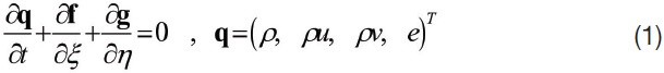
Where
Where,

and

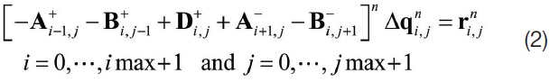
For steady-state problems, the algorithm can be recovered to Newton’s method applied for nonlinear elliptic partial differential equations by neglecting the first term of the right-hand side of equation (4) as an approximation using an infinitely large time step. However, the term is not neglected generally for the diagonal dominance of the matrix solution algorithms.
The equation (2) constitutes a closed set of linear algebraic equations Ax=b for (4×imax×jmax) variables. The matrix A is a block penta-diagonal matrix composed of (4×4) block matrices and strides of imax and jmax. The general procedure for the solution of the linear equations is 1) construct a vector b, 2) construct the matrix A and 3) put A and b into the solver of linear algebraic equations. Thus, a good way of constructing a performance optimized code is 1) construct A and b with BLAS and 2) put A and b into the solver composed with BLAS. However, there is no numerical library for the solution of block penta-diagonal matrices having of arbitrary stride, because the iterative methods can be efficient in this case instead of an exact solver. Moreover, the exact solver is not always necessary, because the matrix A is a temporarily assumed value, and the iterative method is inevitable due to the inherent nonlinearity of the fluid dynamic equations.
The first candidate of the iterative method is the ADI (Alternating Direction Implicit) method. By applying Beam- Warming approximation, the penta-diagonal equations can be replaced by a number of tri-diagonal equations in each direction. The ADI method is widely used because of the existence of an efficient solution algorithm for tri-diagonal equations. Although the ADI method is one of the iterative and approximate methods, sub-iterations are rarely used between iterations even in case of unsteady problems because of the relatively small approximation error. Therefore, the ADI method would be a good choice for the solution of fluid dynamic equations if there were optimized libraries for the tri-diagonal equations. For incompressible flows, the SIMPLE (semi-implicit method for pressure linked equations) algorithm with the ADI method can be a good choice for constructing an efficient code, because all the fluid equations are segregated and a tri-diagonal solver developed with BLAS and included in LAPACK [15], can be used directly. However, the coupled method used for compressible flows results in a block-tri-diagonal system, for which an efficient solver is not yet developed using BLAS.
In the meantime, other iterative methods such as the Jacobi method or Gauss-Seidel’s methods are used in CFD. The Jacobi method has been used for its simplicity in vectorization, but Gauss-Seidel’s method is used more widely for better convergence. The LU-SGS scheme is an improved version of Gauss-Seidel’s method, which has been widely used for the last decade. The procedure of the LU-SGS scheme can be summarized as the following lower and upper sweeps by alternating the direction of the Gauss- Seidel sweeps.


Equations (5) and (6) cannot be vectorized and the (4×4) matrix should be inverted locally. However, those equations can be vectorized if an approximate splitting of the flux Jacobian matrix is applied using spectral radius, a maximum
eigenvalue of the Jacobian matrix.
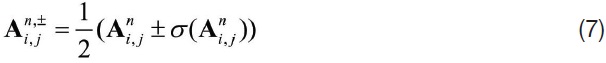
Then the left-hand sides of equation (5) and (6) become a scalar value, and the vectorization can be carried out using the list index along the diagonal direction of computational grid. The LU-SGS algorithm had been developed originally for vector-type supercomputers, but has also been used widely on microprocessor-based systems, including workstations and PCs because of its simplicity and good convergence. The present study will suggest a way of optimizing the LU-SGS method for the architecture of microprocessor systems.
4.2 Basic LU-SGS Solution Procedure
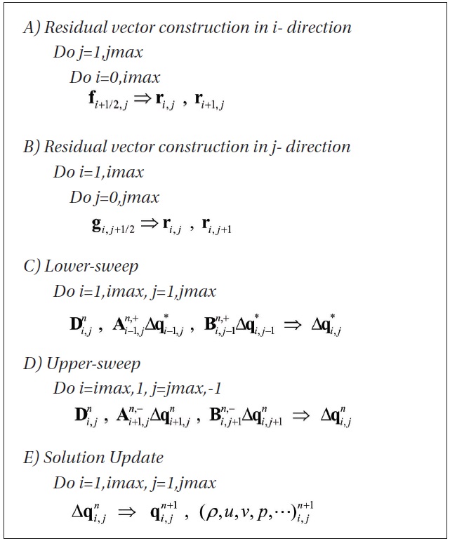
The elementary procedure for the solution of algebraic equations is 1) evaluation of the residual vector and coefficient matrix and 2) put them into the solution library. However, in fluid dynamics, the coefficient matrix is evaluated when it is necessary, because the storage of the block penta-diagonal coefficient matrix is quite large. In case of the LU-SGS algorithm the coefficient matrix is evaluated locally and the solution procedure can be summarized as the following five loops for global variables.
[Algorithm Level 0] Algorithm Level 0

Algorithm Level 0
The first and second steps are the construction steps of the residual vector from primitive variables. The numerical fluxes are calculated at the surfaces, and summed as a residual. The numerical fluxes are added to both sides of residual vectors. These steps require a lot of numerical operations and take a lot of computing time, because the interpolation of variables, limiter functions and eigenvalue corrections are necessary in addition to the calculation of numerical flux functions.
The next step is the lower sweep. This step can be done easily by scalar-inversion, after calculating the product of the split Jacobian matrix and the difference of the conservative variable vector. This procedure can be simplified, and a lot of computing time can be saved by using an analytic form of the product [16]. The upper sweep can be done similarly to the lower sweep in opposite direction. The final step is for the calculation of new conservative variables from the variations and the evaluation of new values of primitive variables from the conservative variables.
The localization, an approach of increasing the utilization of variables read from the main memory, results in reducing the number of loops for global variables. For example, if there were several loops requesting global variables and the size of the array for the global variables is quite large in comparison with the size of data cache, a variable cannot be stored in the cache when it is necessary in a next loop, and the variable should be taken from the main memory. Since there is latency in taking a variable from the relatively slow main memory, the processor becomes idle during that time and the time is not necessarily wasted.
However, if the number of loops can be reduced while maintaining the same results, i.e., maximizing the use of a variable read from the main memory, then the number of access to the main memory can be reduced, and the wasting time can be saved. Therefore, the localization is equivalent to reducing the number of loops, and the overall structure of the code is changed into the computation for local variables with a minimum number of loops. Reduction of the five loops in Algorithm Level 0 will be discussed in the following.
[Algorithm Level 1] Algorithm Level 1
Algorithm Level 1
4.4 Localization
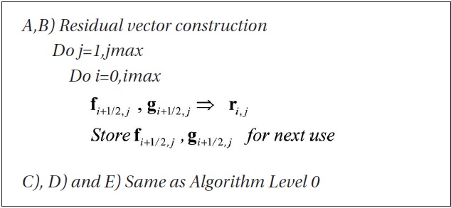
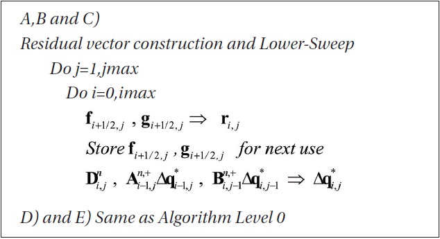
As a first step of reducing the global loops, the merge of step A) and B) can be considered. For A) and B) steps, a variable at a grid point is called twice. However, these two loops can be merged into a single loop by calculating the right and upper numerical fluxes at a time. After that the numerical fluxes should be stored temporarily for the next use. If the i-direction is the inner loop while j is the outer, the right numerical flux is used as the left numerical flux for the next grid point and only four real variables (1×4×8=32 Byte) are necessary. However, the upper numerical fluxes of entire grid points in j-th row should be stored for a while before it can be used as a lower numerical flux for the upper grid point. Although the size of memory is dependent on the I-directional grid point, it is relatively small in comparison with a typical cache size of 256KB. Since a 32 Byte is necessary for a numerical flux, it is thought that more than 1,000 numerical fluxes can be stored for next use, while even considering the other variables. Thus, the number of access to the main memory can be reduced, and some amount of time can be saved as such. Also, it is inevitable to proceed to the next step. The localization algorithm level 0 can be summarized as follows.
4.5 Localization
The second step of localization is the merge of the residual construction step and lower sweep as algorithm Level 2. Since the residual vector is no longer necessary after the lower sweep, it is not necessary to store the residual vector as global variables, but the residual can be stored as only four temporary variables. Thus, a large amount of memory, corresponding to imax×jmax×32 Byte or 20 to 30 % of overall memory, can be saved as an additional effect. As major effects, 1) it does not become necessary to access the residual vector and primitive variables stored in main memory for the lower sweep, and 2) the available cache size can be significantly increased by removing the unnecessary storage of the residual vector in data cache.
[Algorithm Level 2] Algorithm Level 2

Algorithm Level 2
4.6 Localization
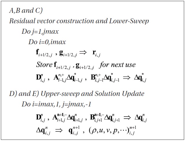
As a next step, the upper-sweep and the solution update procedure can be merged as algorithm Level 3. All the numerical procedure for a grid point is terminated after the upper-sweep, and a new solution can be reconstructed immediately after the upper sweep. Thus, the merge of the upper sweep and the solution update procedure is aimed to reduce the time for taking a variation of a conservative variable from the main memory for reconstruction of new variables. In this case, the solution reconstruction is done in the opposite direction of the lower-sweep since the upper-sweep proceeds in the opposite direction of the lower sweep.
However, the upper-sweep of the original LU-SGS scheme in equation (6) is changed to equation (8), because the variables used for the calculation of the split Jacobian matrix for the next grid point is already updated. Thus, there is a possibility of changing the convergence characteristics, but its effect would always be negative, because the basic concept of Gauss-Seidel’s method is the use of recently updated variables for the calculation of the coefficient matrix.

Following the localization procedures, the five loops in the algorithm Level 0 are reduced to only two loops in the algorithm Level 3. Thus, the access to the main memory can be reduced and the utilization of a variable taken from a main memory can be increased. In other words, the cache hit-ratio can be increased by the frequent use of a variable that is stored in a high-speed temporary location. The next chapter will show the efficiency of the localization algorithms for several problem sizes.
[Algorithm Level 3] Algorithm Level 3
Algorithm Level 3
5. Application of Localization Algorithms
5.1 Test Problems and Environments
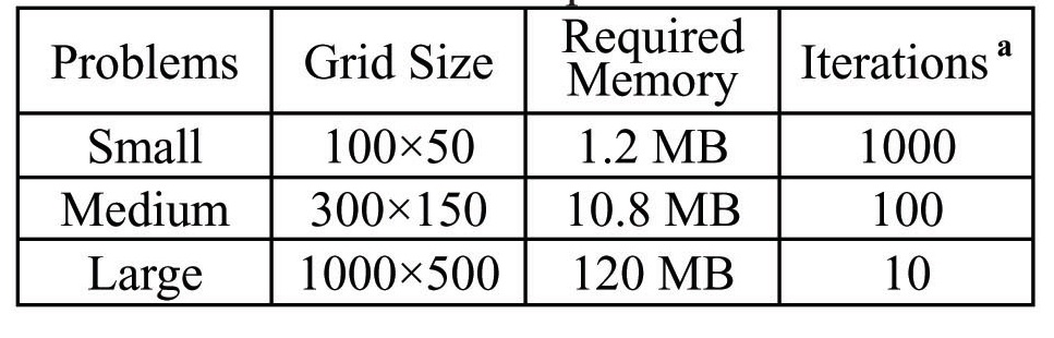
For the examination of the localization algorithms, an inviscid compressible flow problem was considered. The test problem is the numerical solution of Mach number 3 flows over a two-dimensional wedge of a 10 degree turning angle exhibiting an oblique shock wave and expansion waves. Since most of the numerical algorithms can produce sufficiently good solutions, only the convergence characteristic and the time efficiency were examined. In this study, influences by the size of the problem, processor type and compiler was investigated. The sizes of problems were summarized in Table 1.
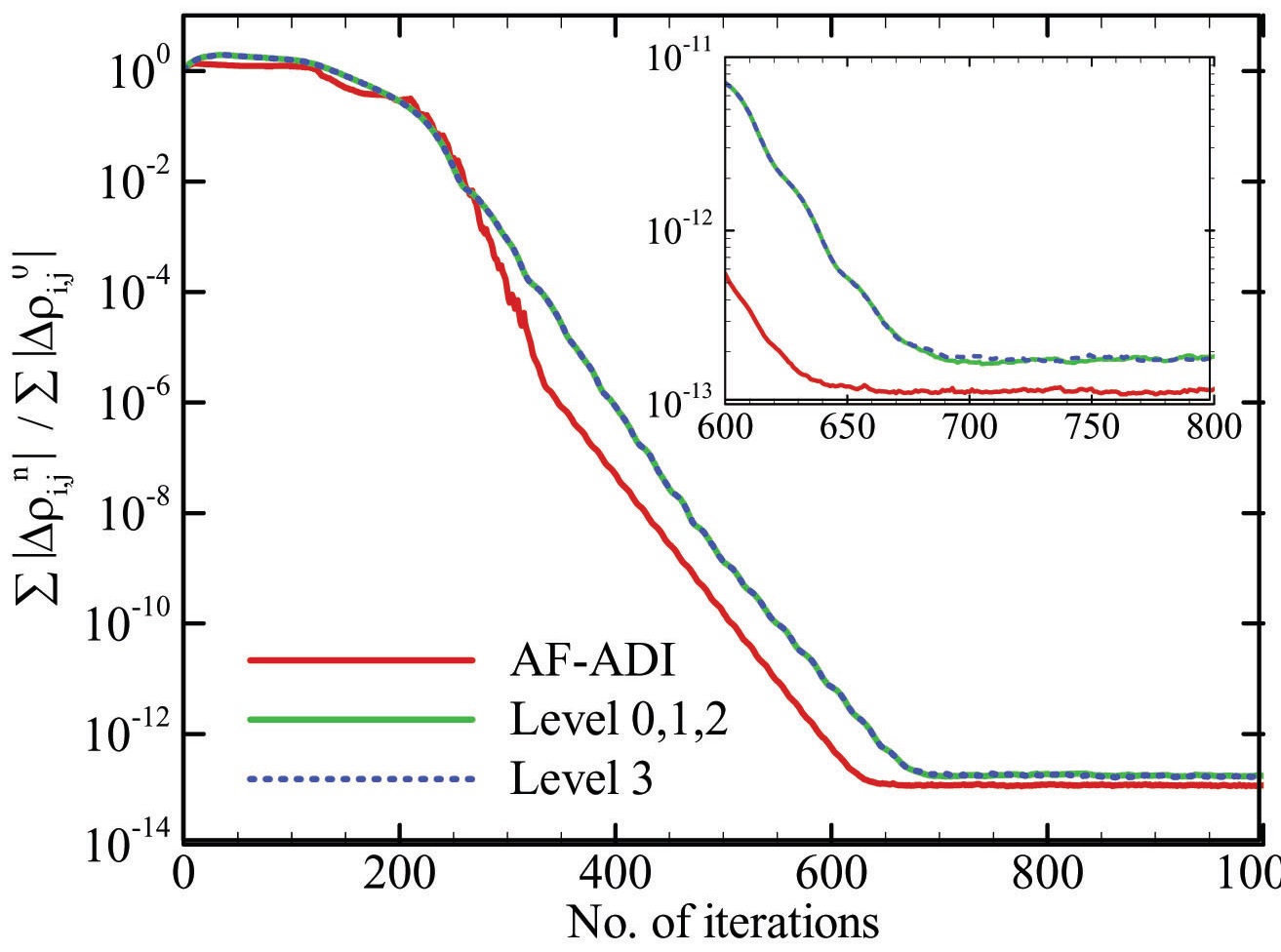
Fig. 3 is the convergence history up to the machine accuracy for a small problem showing the convergence characteristics. Solution by the AF-ADI method is also included for comparison. Since the algorithm Level 0, 1 and 2 are mathematically identical the convergence histories are exactly the same, as well as the solutions. Only the algorithm 3 is slightly different, as described in equation (8), but Fig. 3 does not show any noticeable differences. There is only a slight difference after the machine accuracy is attained. Also, the number of mathematical operations is exactly the same for all the algorithms.
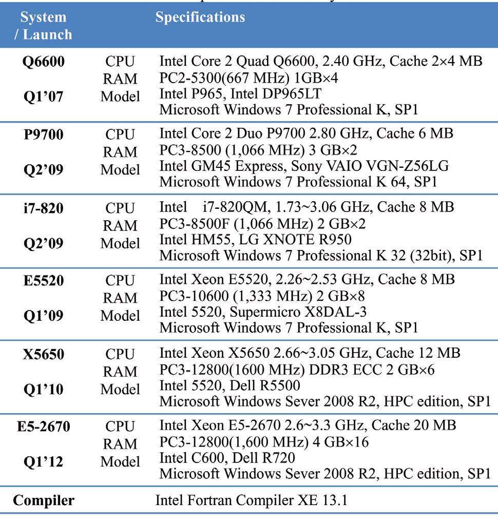
The time consumed for the iterations in Table 1 is measured without the console and disk output. The computing time is measured by using the intrinsic functions such as CPU_TIME() or SECNDS(). All the specifications of the tested computers are summarized in Table 2 including

Test problems
the processor type, cache size, main memory, main board/ chipset, operating system, compiler and compile options. “Q6600”, “P9700” and, etc. are the abbreviation of each system based on the model number of the processor. The time of the processor launch is listed below the title of the system to reflect the advances in processor architectures. Optimal compile options for various systems have been used by the Polyhedron Inc. for the compiler comparison(Unclear) [17].
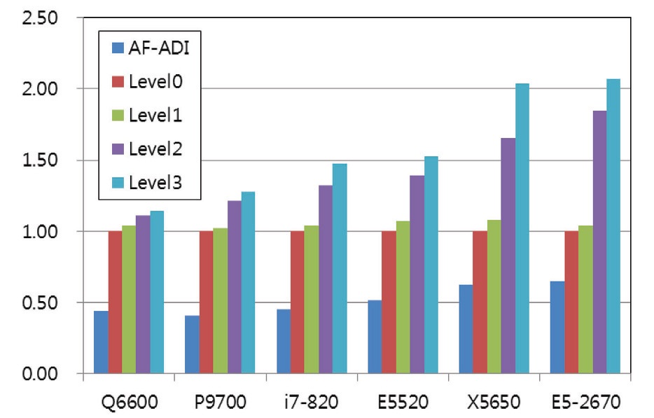
The computing time by the localization algorithms were examined for three problems on several systems. The results of AF-ADI methods are included for ‘Small’ and ‘Medium’ problems for comparison, but cannot be done for large problem since the method requires much larger memory than the LU-SGS scheme. Speed-Up is the ratio of computing time compared to algorithm Level 0, and is summarized in Table 3 to 5, as well as the computing time. The performance of each system is compared visually in Fig. 4 to 6 by using relative speed. Relative speed is the ratio of computing time compared to algorithm Level 0.
5.2 Test Results for ‘Small’ Problems
Various analyses may be possible from the results in Fig. 4 to 6 and Table 3 to 5, but the primary one will be the comparison of algorithms depending on the problem size. The ‘Small’ problem uses a relatively small grid, which requires 1.2 MB of memory. The 1.2 MB memory is very small in comparison with the overall size of main memory and is smaller than the cache memory of the tested systems.
[Table 2.] Specification of test systems and compilers with compile options
Specification of test systems and compilers with compile options
Referring to Fig. 4 and Table 3, the computing time of LU-SGS algorithm is about half of the AF-ADI method depending on each system. For Q6600 systems, the speed-up by the algorithm change is limited to 6% maximum, but the E5520 system shows about a 70% improvement. A point to notice is that the recent processors show much more performance gains, though there is a dependency on each system. This implies inversely that new processor architectures show improved performance gain by the algorithm optimization. However, overall, the performance gain is not as big as expected from the previous studies [4]. It is because the speed of memory becomes several times faster than before, but the clock speed of the processors is maintained around 2~3 GHz.
[Table 3.] Computing time [s] and Speed-Up for Small problem
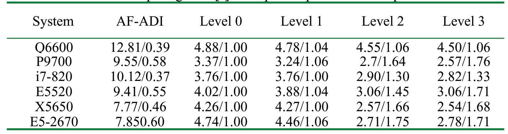
Computing time [s] and Speed-Up for Small problem
[Table 4.] Computing time [s] and Speed-Up for Medium problem
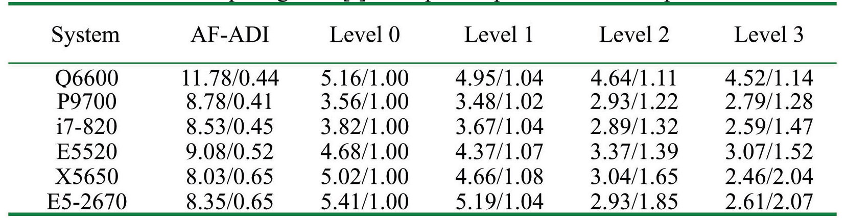
Computing time [s] and Speed-Up for Medium problem
[Table 5.] Computing time [s] and Speed-Up for Large problem
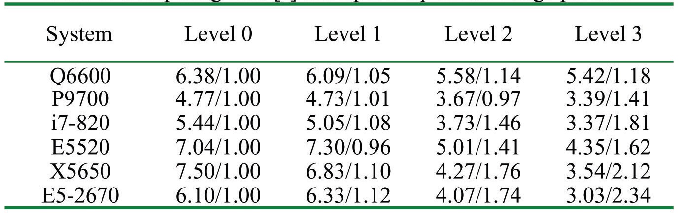
Computing time [s] and Speed-Up for Large problem
Nonetheless, the present results for a small problem does not fully reflect the advantage of the localization techniques, since the problem size is too small and the cache hit ratio would be quite high for most of the systems, i.e. the problem could be handled with the capacity of cache memory.
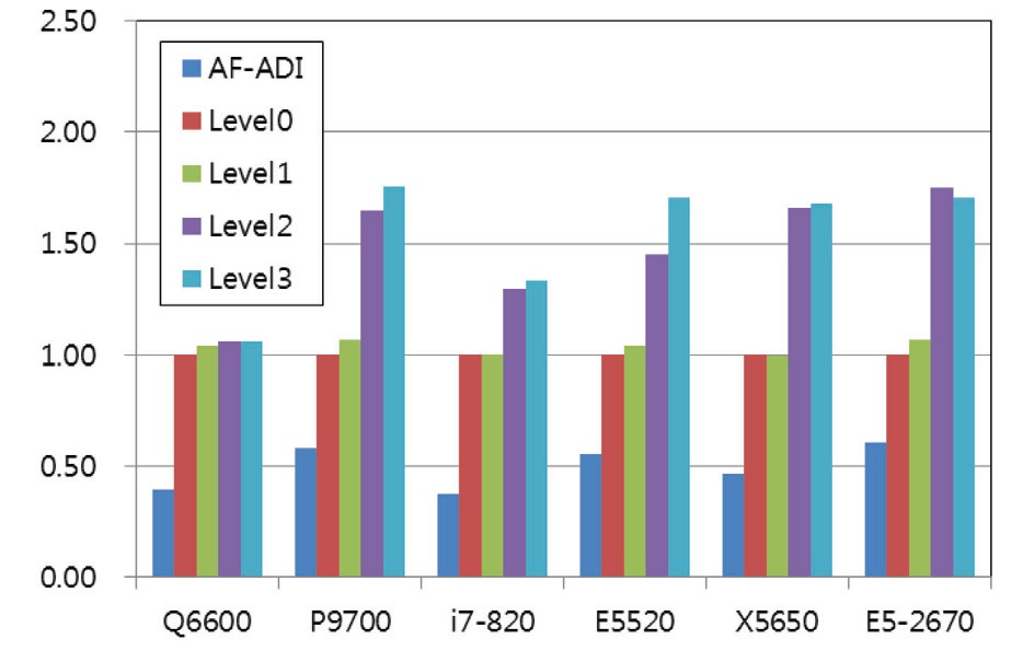
5.3 Test Results for ‘Medium’ Problem
The medium problem asks for 10.8 MB memory, which is greater than the typical cache size of tested systems. The results for the medium problem are summarized in Fig. 5 and Table 4. The results clearly show the advantage of the localization technique for all the systems. Among the various levels, the advantage of the Level 2 algorithm is most
significant. It is reasoned that the advantage comes from two factors. The first one is that the storage of the residual vector is no longer necessary as a global variable, which results in the significant reduction of memory requirement and the increase of cache hit ratio by the availability of cache capacity. The second is that the residual is used for the lower sweep as soon as it is computed, rather than stored for later use in a separate lower sweep, as is for the level 0 and 1. The maximum performance gain is greater than twice that obtained for the latest systems. It is considered that the advantage of the algorithm is greater for the latest systems which have a higher maximum frequency.
5.4 Test Results for ‘Large’ Problem
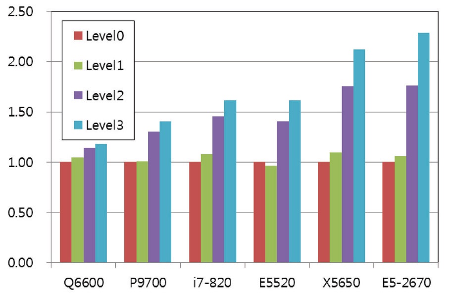
Fig. 6 and Table 5 show the test results for a large problem. This problem requires 120 MB of memory which is much larger than the cache capacity of all the systems tested. The trend is similar to that of a medium problem, but the advantage of the localization is much greater. The advantage of the level 3 algorithm is also shown clearly in these results. Thus, it is considered that the reduction of the global loop is advantageous to improve the computing performance by reducing the access to main memory while increasing the cache hit-ratio. The maximum performance gain by the level 3 algorithm was 2.34 times the level 0 algorithm to obtain the identical solution by the E5-2670 system. It is also shown that the localization technique is advantageous to the latest processors for which the difference of clock speed between the memory and processor is larger.
5.5 Summary of the Effect of Algorithm Improvements
The results in Fig. 4-6 and Table 3-5 show the overall performance improvement according to the increasing the level of localization, even though the amount of performance improvements is dependent on the problem size and system characteristics. Overall, there is no big improvement in level 1 compared to level 0. The performance improvement comes from reducing the number of access to the primitive variables and the residual vector. Level 2 shows significant improvement compared to level 1. Since the change from level 1 to level 2 has combined effects; 1) accessing the residual vector and primitive variables stored in main memory for the lower sweep becomes unnecessary, and 2) the available cache size can be significantly increased by removing the unnecessary storage of the residual vector in data cache. A simple correction level 3 has a relatively significant improvement due to the small overall computing time, although the absolute saving is quite comparable to that of level 1 from level 0. These results support the reasoning of developing the localization algorithms.
In addition to the algorithms, characteristics of the computing systems can be understood as well, and the comparison between the computing systems is feasible. The latest processor architectures show the strong dependency on algorithm optimization. However, Q6600, relatively old processor architecture, was less sensitive to algorithm optimization, although there is a dependency on problem size.
The latest microprocessor systems have a large performance gap between the microprocessor, and the main memory, and high-speed cache is employed to cover the gap. Therefore, the performance of a numerical code is dependent on the algorithms that can maximize the utilization of variables taken from main memory while reducing the access to the main memory. This is equivalent to reducing the number of loops for global variables and has the effect of increasing the cache hit-ratio.
In the present study, methods for improving the performance of a code for the LU-SGS scheme were verified in several levels based on the reasoning of the latest microprocessor architectures. The improvements of the algorithms were examined for several of the latest micro processor systems regarding numerous problem sizes. The results exhibit clear performance improvement by the code optimization, called here as localization. Although the magnitude of improvement is dependent on problem size and system architectures, the performance improvement was monotone according to the level of localization, regardless of system architectures. A solution more than twice as fast was obtained at the same computer system (Unclear) for producing the exact same solution with the same number of floating-point operations.
From the present results, it is shown that the latest microprocessors having higher operation speeds are much more sensitive to localized algorithms. Also, it is shown that the processor speed does not guarantee the higher performance, unless the computational code is optimized for the memory hierarchy. Therefore, it is concluded that the code optimization on the memory hierarchy of the latest microprocessors is no longer a matter of choice, but a compulsory subject.


![Computing time [s] and Speed-Up for Small problem](http://oak.go.kr/repository/journal/12081/HGJHC0_2013_v14n2_112_t003.jpg)
![Computing time [s] and Speed-Up for Medium problem](http://oak.go.kr/repository/journal/12081/HGJHC0_2013_v14n2_112_t004.jpg)
![Computing time [s] and Speed-Up for Large problem](http://oak.go.kr/repository/journal/12081/HGJHC0_2013_v14n2_112_t005.jpg)