The water system plays an important role as a lifeline for our existence. It is through pipelines that water is distributed to customers for steadiness and safety. Water pipes, however, tend to be corroded as time goes by. Pipes laid underground are hardly examined without excavation. Some deteriorated pipes may be exposed to leakage or damages, resulting in the decline or interruption of water supply. In order to maintain customer service at a desirable level, replacement of such old pipelines is considered inevitable. As the replacement of pipelines requires huge costs and time, there is a pressing need to provide information on how to evaluate the pipe condition in an effective way.

Deterioration or corrosion of pipes may cause cracks and bursts, resulting in water leakage, pipe repair, and poses even the so-called water quality problem ‘red water’. Occurrence of the corrosion relates to many factors: pipe materials, pipe age, surrounding soil conditions, water quality, pipe maintenance and management [1,2]. It is, therefore, difficult to examine where the corrosion is taking place and the extent of it. Corrosion of the outer surface of the metallic pipes occurs mainly due to electrochemical reactions under the heterogeneous soil condition. The reaction rate is influenced by soil resistivity, permeability and mineral ions existing around the installed pipes [3,4].

Most of the previous researches dealt with causual analysis of pipe corrosion and prediction of future corrosion for water distribution pipes. Katano et al. [5] found the log-normal distribution fit their pit data the best and analyzed environmental factors using regression analysis. The environmental factors (soil type, pH, resistivity, redox potential, and sulfate ion) were found to be significant in determining pit depth. Kolovich and Kiefner [6] developed the Monte Carlo method for determining the corrosion rate distribution in buried pipelines that uses the probability distributions of corrosion depth and initiation time. Restrepo et al. [7] employed statistical techniques like cluster analysis to establish the sampling design and later for data analysis and obtaining a mathematical expression for external corrosion depth as a function of several experimental variables [7]. In addition, various studies have reported different methodologies used to be able to predict the future trend of corrosion for water pipeline.

The present study has strengths that although data is insufficient, effective evaluation of the current condition and prediction model can obtain a clear quantitative model by statistical approach and application is easy in other areas because of high reproducibility. In order to obtain a quantitative model for measuring pipe corrosion, we propose to apply an evaluation index to fuzzy environmental soil conditions around water pipes.

The present study aims at proposing an approach and method to predict the intensiveness and probable points of pipe corrosion in the pipe network. Base data utilized for the prediction are those sampled at the site. Objectives of the study are referred to: 1) obtain evaluation indexes for external corrosion reflecting the fuzzy soil nature of installation sites; 2) develop a multiple regression model to measure the degree of pipe corrosion under the fuzzy soil conditions; and 3) evaluate future risk and timing for decision of pipeline replacement.

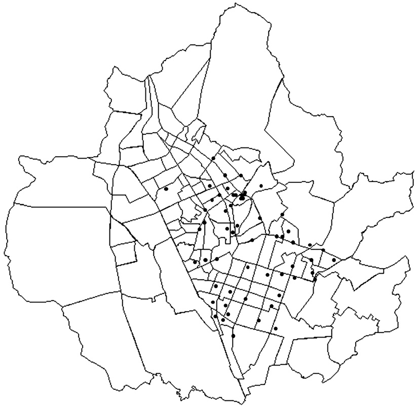
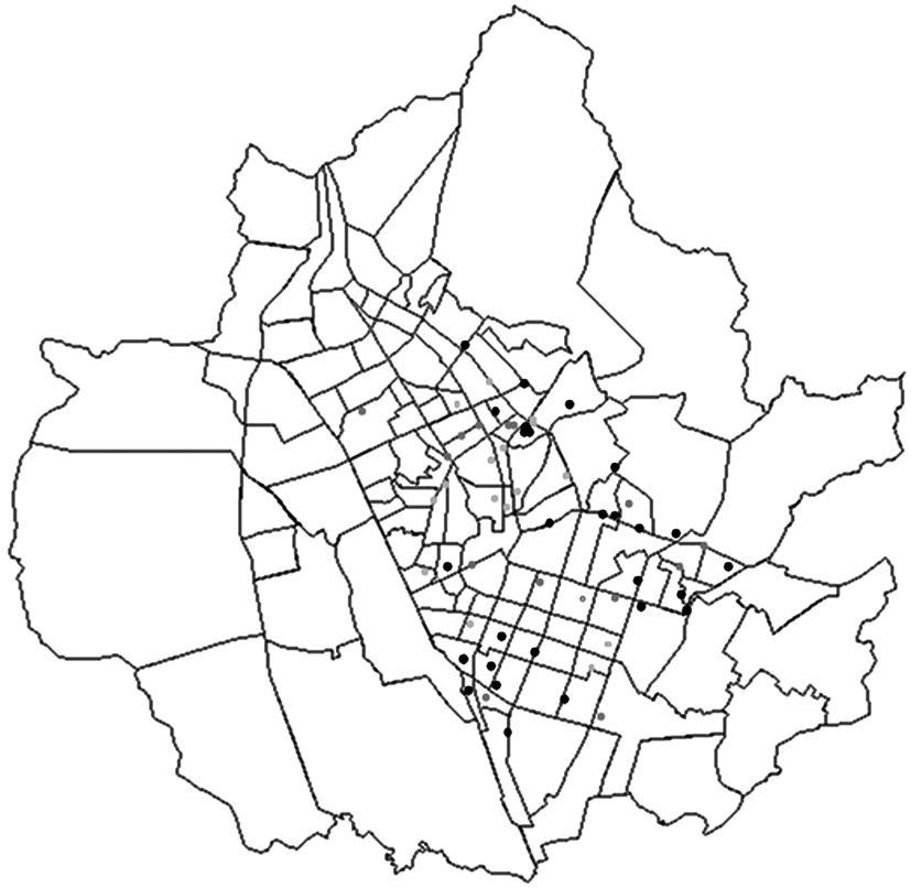
The study focuses on the existing distribution pipe network in S city, South Korea during 2009？2010 [8]. Field data on pipe corrosions and soil conditions around pipes were obtained in the previous research project including those of the test pit excavation at 60 random locations along the water distribution pipelines (Fig. 1). The study area extends to 121.05 km² with a population of approximately 1.11 million [9].

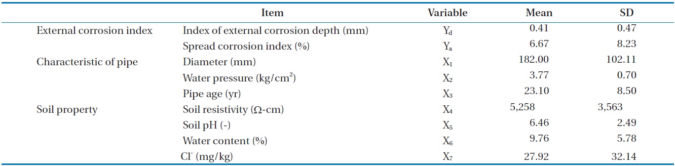
Table 1 shows relevant data for this analysis with their mean values and standard deviation. The external corrosion is measured by two indexes: external corrosion depth given as localized corrosion index (Y_d), and corrosion spread on the pipe’s surface given as general corrosion index (Y_a). Influential factors are grouped into two: factors related to ‘characteristic of water pipe’ and ‘soil condition’. The former contains 3 items, all of which are obtained from geographic information system (GIS) database of the distribution pipe network. The latter are 4 items as measured from soil sample testing.

The previous studies suggest synergistic effect of the external corrosion depth (Y_d) and the corrosion spread (Y_a) on pipe breakage [10]. Following the spread of general corrosion, the localized corrosion may occur at a specific point on pipes coincidentally. So we have analyzed these two types of corrosion in parallel.

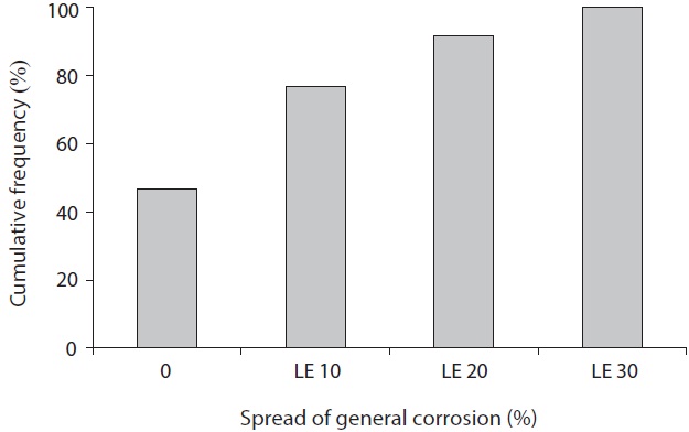
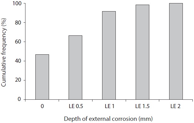
Prior to the main analysis, corrosion conditions are presented in histograms to show cumulative frequency vs. corrosion level (Figs. 2 and 3). No pipe corrosion is found at 47% of randomly selected sample points. Despite the pipe age of 12 to 52 years, some newer pipes (under 20 years) have deeper and/or wider spread of corrosion than the average. To the contrary, there are some uncorroded samples found in older (over 40 years) pipes. This tendency is considered to be closely related to characteristics of the surrounding soil conditions and the pipe conditions which are not protected by a polyethylene sleeve. Next, histograms are created for each of the soil properties in order to make it easy to understand a distribution of samples

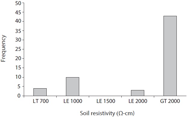
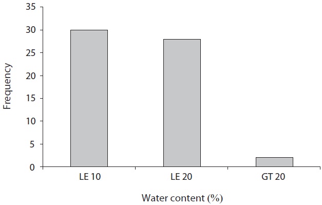
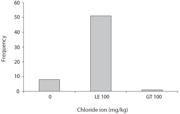
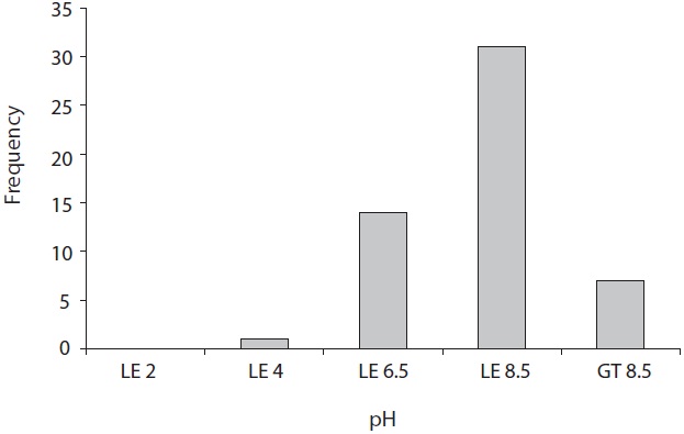
(Figs. 4？7). For soil resistivity, it was identified by the American National Standards Institute (ANSI) method that only four samples had measurement values below 700 to be under the very highly corrosive soil condition, and around 72% of samples indicated values above 2,000 to be sampled from the extremely low corrosive soil condition. As pH’s histogram shows, also, only one sampling point had acidity of less than 4, whereas 7 sampling

points were found to have alkalinity of over 8.5. Next, in relation to water content, exactly half the samples is obtained from dry contition (water content is less than 10%). Lastly, chloride ion was detected from 87% of soil samples. These figures illustrate that the sampling points covered a wide range of soil conditions.

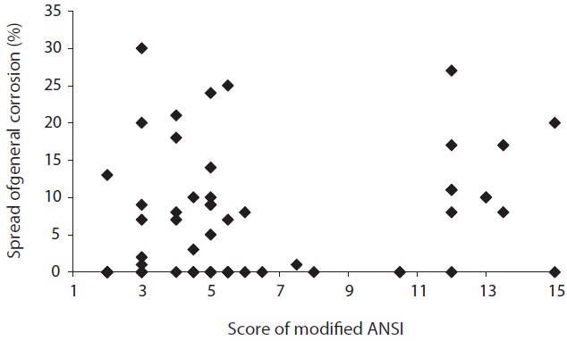
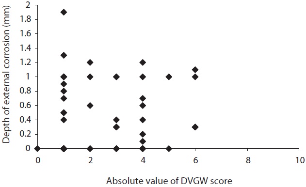
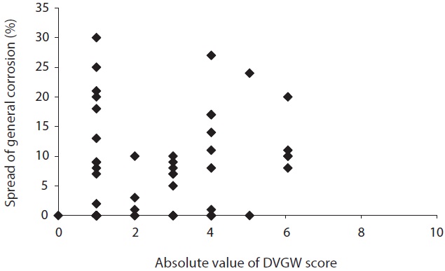
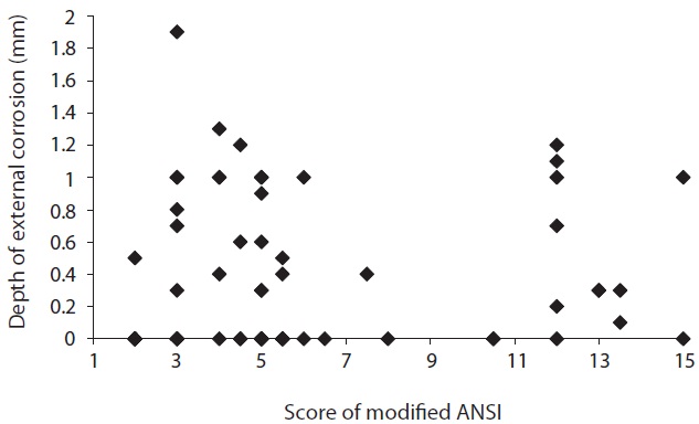
Then, the corrosive condition of soil samples was evaluated using the modified ANSI method and the German Waterworks Association (DVGW) method which are the most representative

methods for evaluation of soil corrosivity. As the results, nearly 47% of soil samples were evaluated as the corrosive condition (middle and strong corrosivity) by the modified ANSI method. On the other hand, around 88% of soil samples were found to be evaluated as weak corrosivity and 12% soil samples as middle corrosivity using the DVGW method. Also, the relation between the corrosive condition of each soil sample was evaluated by two methods and the actually measured external corrosion is shown in Figs. 8？11. As Figs. 8 and 9 illustrate, there are samples that actually measured external corrosion depth and spread of general corrosion have low values with the high score of modified ANSI and also have high values with the low score of modified ANSI. Similarly, between actually measured values of external corrosion and absolute values of DVGW score don’t have definite relationship as shown in Figs. 10 and 11. These results mean that there are significant differences between the actually measured external corrosion and the corrosive condition evaluated by the two methods above. Thus, it is considered that a new evaluation method of corrosivity regarding soil samples should be developed.

In this study, in order to obtain a more reliable model to predict the degree of pipe corrosion, the relationship between external corrosion and soil property is further investigated by applying discriminant function analysis (DFA). From examining the discriminant function, we quantify the soil environment corrosivity using some combination of variables in which the

fuzzy soil property is reflected. The multiple regression model (MRM) is to measure the degree of pipe corrosion. In developing MRM, some of the pipe characteristics are considered effective as explanatory variables together with the selected variables in the DFA. By developing the MRM, the degree of pipe corrosion at some points is predicted for evaluation of present and future risk.

In order to distinguish the corrosive soil environment in all soil samples, DFA is applied to this analysis. Common purpose of the DFA is to predict the group membership based on a linear combination of variables using a measure of generalized square distance assuming that each group has a multivariate normal distribution. Another purpose of DFA is to acquire insight into the relationship between the group membership and variables in the prediction model which is given as a discriminant function.

At the beginning of DFA, observations for each group are made including both high-ranking and low-ranking samples reflecting a characteristic of the universe (the population of all samples). In this study, two groups, namely, a corrosive group (named BAD group) and a non-corrosive group (named GOOD group) are considered for each discriminant function corresponding

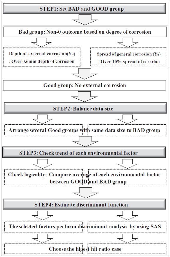
to each corrosion indexes (Y_d and Y_a). The modeling process with the discriminant function is proposed in the following order as shown in Fig.12.

Step 1. Set sample condition for BAD and GOOD group

It is a normal procedure that DFA focuses merely on data ranked high and low (namely, the first quarter and the last quarter of the sorted samples). In this study, 16 samples (almost the last quarter) which had over 0.6 mm of corrosion depth are regarded as the BAD group corresponding to Yd, and 12 samples with over 10% area corrosion are categorized into the BAD group corresponding to Ya. On the other hand, the GOOD group consists of no external corrosion samples both for Yd and Ya. As the numbers of effective data differ between these groups, a measure to balance the sample data is required.

Step 2. Balance sample size between BAD and GOOD group

To ensure stability of DFA, two groups are preferably equal in data size. As the number of samples in the GOOD group is greater than sample size of the BAD group, random sampling methods are adopted to select samples for the GOOD group. Several sets of samples are arranged so that the Good group may have same sample size to the BAD group, and then the corresponding models for classification are examined as below.

Step 3. Examine whether each environmental factor is logically acceptable

After adjusting the sample size of both groups, the average value of each environmental factor for each group is compared. When the average value of an environmental factor in the BAD group is higher than that of the GOOD group, such a factor is judged to have logicality, excluding soil resistivity (X4), which has the opposite tendency.

Step 4. Estimate discriminant function

The DFA model is developed with the aid of SAS ver. 6.03 (SAS Institute Inc., Cary, NC, USA) as a function of the selected factors, logically reasonable. For depth of external corrosion (Yd) and spread of general corrosion (Ya), 5 randomly sampled cases are analyzed respectively. The most reliable DFA models are selected for Yd and Ya which have the highest hit ratio, respectively.

As for external corrosion depth (Y_d), equations obtained from the analyses are assessed as highly reliable. Eq. (1) represents a linear discriminant function. If a classification index (Z_d) estimated from this equation is greater than zero, it is considered that the sample falls into the GOOD category. This implies the external corrosion depth within the range of less than 0.6 mm. Explanatory factors (X₄ and X₆) are standardized as expressed in Eqs. (2) and (3), respectively. Table 1 shows their mean values (m₄ and m₆) and standard deviations (s₄ and s₆). From coefficients in the Eq. (1), W₄ has a larger absolute value than that of W₆. This indicates that the soil resistivity (X₄) is more influential than the water content (X₆) on the external corrosion depth.

On the other hand, as for the spread of general corrosion (Y_a), the soil resistivity (X₄) is found as an influential factor. Eq. (4) stands for a linear discriminant function obtained for Y_a. A standardized variable, W₄ in Eq. (4), is similar of the soil resistivity (X₄) as presented in the Eq. (2) above. If Z_a is greater than 0, then the sample is classified to the GOOD group. This implies that the spread of general corrosion is estimated as less than 10% of pipe surface.

Evaluation indexes of fuzzy soil properties can be obtained from the linear discriminant functions. From these indexes, we can assess corrosiveness of the soil properties. It is found that low resistivity and/or high water content of the soil properties accelerate the rate of external corrosion depth. In the case of the general horizontal corrosion, however, the low resistivity of the soil is considered dominant in affecting an extent of the spread area and its corrosion rate. As to external corrosion prediction, regression analysis is applied to find influential factors related to pipe characteristics. Among 60 sampled data, nearly half of the sampled data didn’t find corrosion on pipe surface. To minimize the effects on the regression model, these data are omitted in the succeeding analyses. The number of data utilized is twenty and nineteen samples for external corrosion depth and general horizontal corrosion, respectively.

It is believed that pipe characteristics and soil properties have linear and non-linear effects on pipe corrosion [11]. To incorporate these effects into the analyses on a same basis, this nonlinear effect is first expressed in the form of power regression equations with a variable of pipe characteristics. Then, multiple regression equations for the two types of external corrosion (Y_d and Y_a) are formulated as a function of the selected factors expressed in linear and/or non-linear forms.

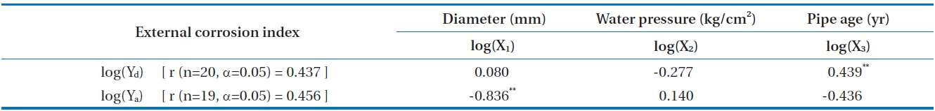
Prior to regression analysis, the correlation coefficient for the logarithmic data of pipe characteristic factors with corrosion indexes are estimated as shown in Table 2. Significant levels of reliability are confirmed as a result of the t-distribution test corresponding to sample size ‘n’ and statistically significant level ‘’. When an absolute value of the correlation coefficient is greater than its significance level, the factors are assessed as statistically significant. In Table 2, the depth of external corrosion (Y_d) has a non-linear relation with pipe age (X₃), and spread of general corrosion (Y_a) with diameter (X₁). These results suggest the effectiveness of adopting each factor as one of the explanatory variables in the corrosion prediction equations.

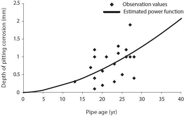
Step 1. Power regression model for external corrosion depth

Firstly, the regression model for between depth for external corrosion (Yd) and pipe age (X3) was made in the form of power function. According to Eq. (5), the estimated power coefficient (1.670) is greater than 1.0. This implies that the pipe age would affect pipe deterioration with acceleration as seen in Fig. 13.

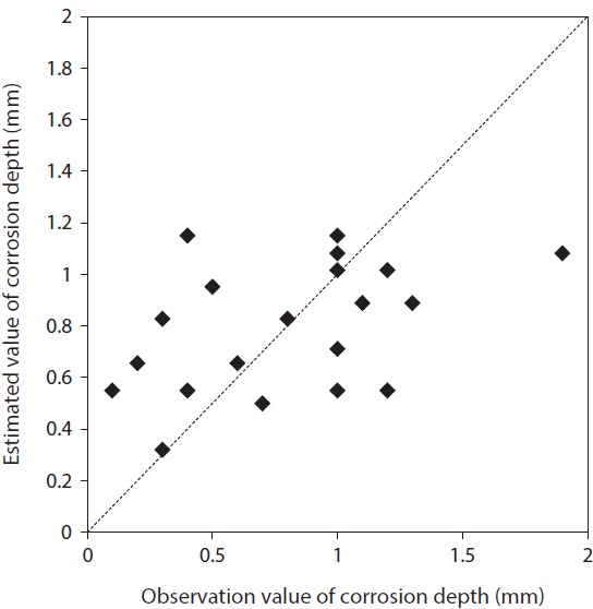
Step 2. MRM for external corrosion depth

Following DFA and regression analysis in the form of power function, multiple regression analysis (MRA) is applied for further analysis. As the explanatory variables, the MRA utilizes pipe age expressed as 1.67th power, soil resistivity (X4) and water content (X6) as previously verified effective by the discriminant function. This regression model expressed in Eq. (6)

is assessed statistically significant from its multiple correlation coefficient (R) obtained through the t-distribution test. The relation between the observed and the estimated values of external corrosion depth is shown in Fig. 14, which indicates sufficient accuracy of our model with a mean absolute error, 0.33 mm.

Step 3. Power regression model for spread of general corrosion

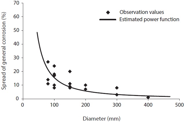
In the same way as stated above, a prediction model for the spread of general corrosion (Ya) is expressed as a factor of the pipe diameter (X1). The negative power (i.e., -1.435) of X1 implies that value Ya (the corrosion spread on pipe surface in percentage) tends to progressively decrease against an increase in value X1 (the pipe diameter). This tendency is clearly seen in Fig. 15.

Step 4. MRM for spread of general corrosion

The main culprit behind the general corrosion is soil resistivity (X4) among soil properties. According to the findings of regression analysis, pipe diameter (X1) is considered to have a negative relation with the general corrosion (Ya). In a multiple regression equation developed here, there are two independent variables as shown in Eq. (8). A correlation coefficient of the equation is estimated at 0.696. As examined by the tdistribution test, this value is able to ensure reliability of the equation.

Severity of the general corrosion for any pipes in the target area can be simply estimated from the equation. Data required for prediction are merely pipe diameter and soil resistivity in the targeted area. The equation is not expressed as the function of pipe age. This is due to the fact that the general corrosion rate per year is rather slower than that of the external corrosion depth. Continuous efforts are required to collect data on pipe corrosion. It may be possible to develop a more reliable prediction model based on the process as mentioned above.

In the previous paragraph, a prediction model for the external corrosion depth (Y_d) represented by pipe age (X₃), soil resistivity (X₄), and water content (X₆) was proposed.

Another method is a prediction which considers the soil environment around the pipes. Corrosion depth of 60 samples in the future is tentatively forecast in the Eq. (6), assuming that the pipes are left without any maintenance for 20 years. In this study a depth of external corrosion over 2 mm is considered serious and may result in pipe damage or leakage. Analyzing the result of forecast, a total of 27 out of 60 samples are expected to have serious external corrosion with a depth exceeding 2 mm on their pipe surface. Locations of those samples are given in Fig. 16. Out of total 60 soil samples, 39 consist of soft clay and 17 of red clay, while 4 samples are of sands. Soft and red clay, accounting for nearly half of the total are causing a rapid growth of corrosion, but the remnants are rather slow in corrosion, as they are predicted not to reach 2 mm. These results indicate that future risk of corrosion closely relates not only to the soil factors but also to the pipe characteristics.

This study intended to predict the severity of pipe corrosion in the target area. The study was carried out through assessment of various data collected at survey points. Results of the analyses indicate that influential parameters on external corrosion depth (Y_d) are soil resistivity (X₄), water content (X₆), and pipe age (X₃). It is also confirmed that the soil resistivity (X₄) and the pipe diameter, among others, affect the spread of general corrosion (Y_a). From all the above, it can be concluded that the multiple regression equation obtained herein provides valuable information on the degree and rate of external pipe corrosion in the target area. The proposed process for future risk evaluation is also effective to decide pipeline replacement and planning. Continuing efforts for collecting and storing up field data are, however, considered important to improve the reliability of the proposed prediction model obtained through statistical analyses.