Let us consider the problem of approximating a divergence
following
A divergence approximator can be used for various purposes, such as two-sample testing [1,2], change detection in time-series [3], class-prior estimation under classbalance change [4], salient object detection in images [5], and event detection from movies [6] and Twitter [7]. Furthermore, an approximator of the divergence between the joint distribution and the product of marginal distributions can be used for solving a wide range of machine learning problems [8], including independence testing [9], feature selection [10,11], feature extraction [12,13], canonical dependency analysis [14], object matching [15], independent component analysis [16], clustering [17,18], and causal direction learning [19]. For this reason, accurately approximating a divergence between two probability distributions from their samples has been one of the challenging research topics in the statistics, information theory, and machine learning communities.
A naive way to approximate the divergence from

and

of the distributions
However, this naive two-step approach violates
If you possess a restricted amount of information for solving some problem, try to solve the problem directly and never solve a more general problem as an intermediate step. It is possible that the available information is sufficient for a direct solution but is insufficient for solving a more general intermediate problem.
More specifically, if we know the distributions
that do not involve the estimation of distributions
The purpose of this article is to give an overview of the development of such direct divergence approximators. In Section II, we review the definitions of the Kullback- Leibler divergence, the Pearson divergence, the relative Pearson divergence, and the
A function
Non-negativity: ∀x, y, d(x, y) ≥ 0
Non-degeneracy: d(x, y) = 0 ⇔ x = y
Symmetry: ∀x, y, d(x, y) = d(y, x)
Triangle inequality: ∀x, y, z d(x, z) ≤ d(x, y) + d(y, z)
A divergence is a pseudo-distance that still acts like a distance, but it may violate some of the above conditions. In this section, we introduce useful divergence and distance measures between probability distributions.
>
A. Kullback-Leibler (KL) Divergence
The most popular divergence measure in statistics and machine learning is the KL divergence [26], defined as
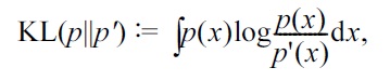
where
Advantages of the KL divergence are that it is compatible with maximum likelihood estimation, that it is invariant under input metric change, that its Riemannian geometric structure is well studied [27], and that it can be approximated accurately via
The PE divergence [30] is a squared-loss variant of the KL divergence defined as
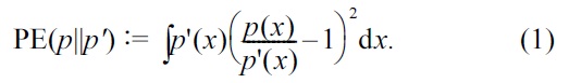
Because both the PE and KL divergences belong to the class of Ali-Silvey-Csiszar divergences (which is also known as
The PE divergence can also be accurately approxi-mated via direct density-ratio estimation, in the same way as the KL divergence [23,28]. However, its approximator can be obtained
>
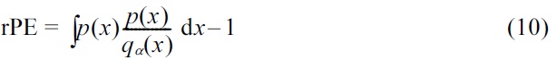
C. Relative Pearson (rPE) Divergence
To overcome the possible unboundedness of the density- ratio function
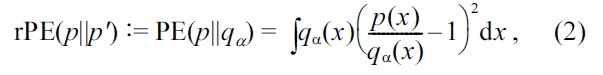
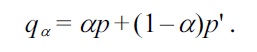
where, for 0 ≤ α < 1,
When
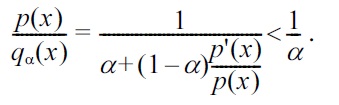
Thus, it can overcome the unboundedness problem of the PE divergence, while the invariance under input metric change is still maintained.
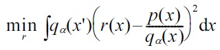
The rPE divergence is still compatible with least-squares estimation, and it can be approximated in almost the same way as the PE divergence via
The
The
The
III. DIRECT DIVERGENCE APPROXIMATION
In this section, we review recent advances in direct divergence approximation.
Suppose that we are given two sets of independent and identically distributed samples
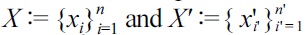
from probability distributions on ?
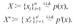
Our goal is to approximate a divergence between from
>
A. KL Divergence Approximation
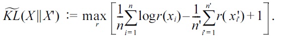
The key idea of direct KL divergence approximation is to estimate the density ratio
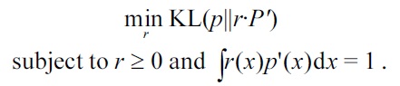
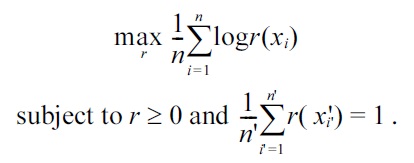
Its empirical optimization problem, where an irrelevant constant is ignored and the expectations are approximated by the sample averages, is given by
Let us consider the following Gaussian density-ratio model:
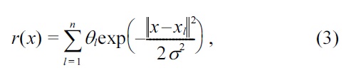
where ||·|| denotes the

as
where, T denotes the transpose. In this model, the Gaussian kernels are located on numerator samples

, because the density ratio
exist. Alternatively, Gaussian kernels may be located on both numerator and denominator samples, but this seems not to further improve the accuracy [21]. When n is very large, a (random) subset of numerator samples
may be chosen as Gaussian centers, which can reduce the computational cost.
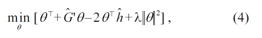
For the Gaussian density-ratio model (3), the above optimization problem is expressed as
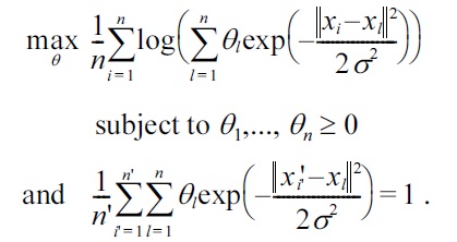
This is a convex optimization problem, and thus the global optimal solution can be obtained easily, e.g., by gradient-projection iterations. Furthermore, the global optimal solution tends to be
The Gaussian width
are divided into

of (approximately) the same size. Then, a density-ratio estimator

is obtained using
(i.e., all numerator samples without
where |
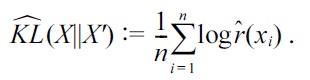
Given a density-ratio estimator

, a KL-divergence approximator
can be constructed as
A MATLABR® (MathWorks, Natick, MA, USA) implementation of the above KL divergence approximator (called the
“http://sugiyama-www.cs.titech.ac.jp/ ~sugi/software/KLIEP/”.
Variations of this procedure for other density-ratio models have been developed including the log-linear model [34], the Gaussian mixture model [35], and the mixture of probabilistic principal component analyzers [36]. Also, an unconstrained variant, which corresponds to approximately maximizing the
>
B. PE Divergence Approximation
The PE divergence can also be directly approximated without estimating the densities
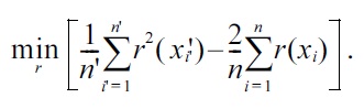
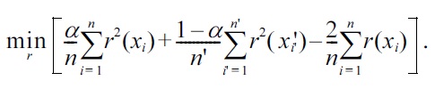
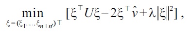
Its empirical criterion, where an irrelevant constant is ignored, and the expectations are approximated by the sample averages, is given by
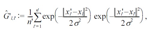
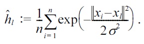
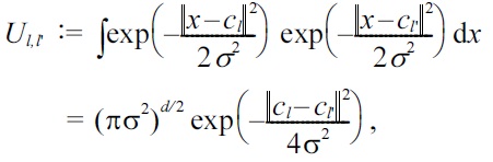
For the Gaussian density-ratio model (3) together with the
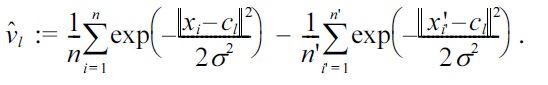
where

is the
and

is the
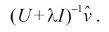
This is a convex optimization problem, and the global optimal solution can be computed
where
The Gaussian width
and

are divided into

and

respectively. Then, a density-ratio estimator

is obtained using

This procedure is repeated for
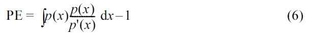
By expanding the squared term
in Equation (1), the PE divergence can be expressed as
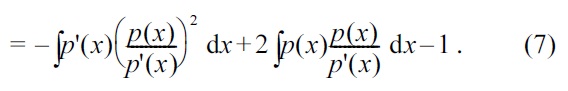
Note that Equation (7) can also be obtained via
as
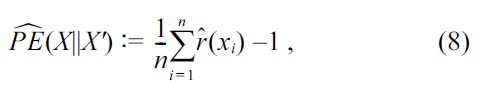
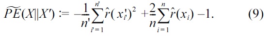
Equation (8) is suitable for algorithmic development because this would be the simplest expression, while Equation (9) is suitable for theoretical analysis because this corresponds to the negative of the objective function in Equation (4).
A MATLAB implementation of the above method (called
“http://sugiyama-www.cs.titech.ac.jp/ ~sugi/software/uLSIF/”.
If the
in Equation (4) is replaced with the
the solution tends to be sparse [39]. Then the solution can be obtained in a computationally more efficient way [40], and furthermore, a regularization path tracking algorithm [41] is available for efficiently computing solutions with different regularization parameter values.
>
C. rPE Divergence Approximation
The rPE divergence can be directly estimated in the same way as the PE divergence [24]:
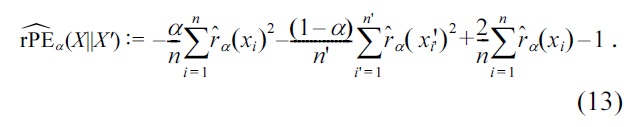
Its empirical criterion, where an irrelevant constant is ignored and the expectations are approximated by sample averages, is given by
For the Gaussian density-ratio model (3), together with the

where

is the
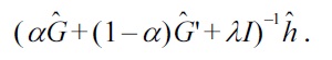
This is a convex optimization problem, and the global optimal solution can be computed analytically as
Cross-validation for tuning the Gaussian width
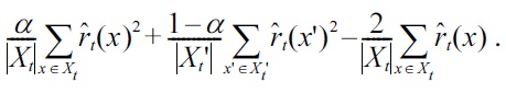
By expanding the squared term
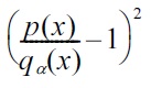
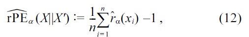
in Equation (2), the rPE divergence can be expressed as

Based on these expressions, rPE divergence approximators are given, using the relative density-ratio estimator

as
A MATLAB implementation of this algorithm (called
“http://sugiyama-www.cs.titech.ac.jp/ ~yamada/RuLSIF.html”.
>
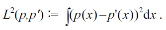
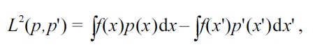
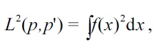
D. L2-Distance Approximation
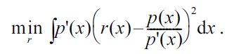
The key idea is to directly estimate the density difference
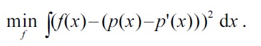
Its empirical criterion, where an irrelevant constant is ignored and the expectation is approximated by the sample average, is given by
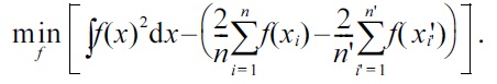
Let us consider the following Gaussian density-difference model:
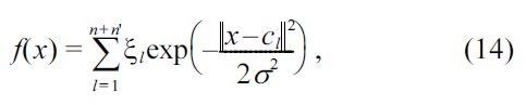
where

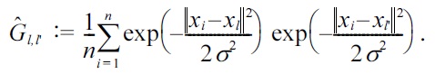
are Gaussian centers. Then the above optimization problem is expressed as
where the

is included,

is the (
This is a convex optimization problem, and the global optimal solution can be computed
The above optimization problem is essentially the same form as least-squares density-ratio approximation for the PE divergence, and therefore least-squares density-difference approximation can enjoy all the computational properties of least-squares density-ratio approximation.
Cross-validation for tuning the Gaussian width
and
are divided into
and
respectively. Then a density-difference estimator
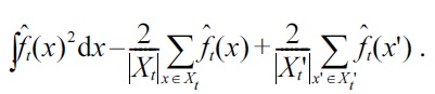
Note that the first term can be computed analytically for the Gaussian density-difference model (14):
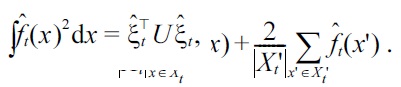
where

is the parameter vector learned from
For an equivalent expression of the
if

, and the expectations are approximated by empirical averages, the following
Similarly, for another expression
replacing
gives another
Equations (15) and (16) themselves give valid approximations to
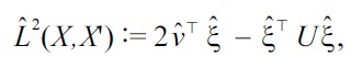
was shown to have a smaller bias than Equations (15) and (16).
A MATLAB implementation of the above algorithm (called
“http://sugiyama-www.cs.titech.ac.jp/ ~sugi/software/LSDD/”.
IV. USAGE OF DIVERGENCE APPROXIMATORS IN MACHINE LEARNING
In this section, we show applications of divergence approximators in machine learning.
>
A. Class-Prior Estimation under Class-Balance Change
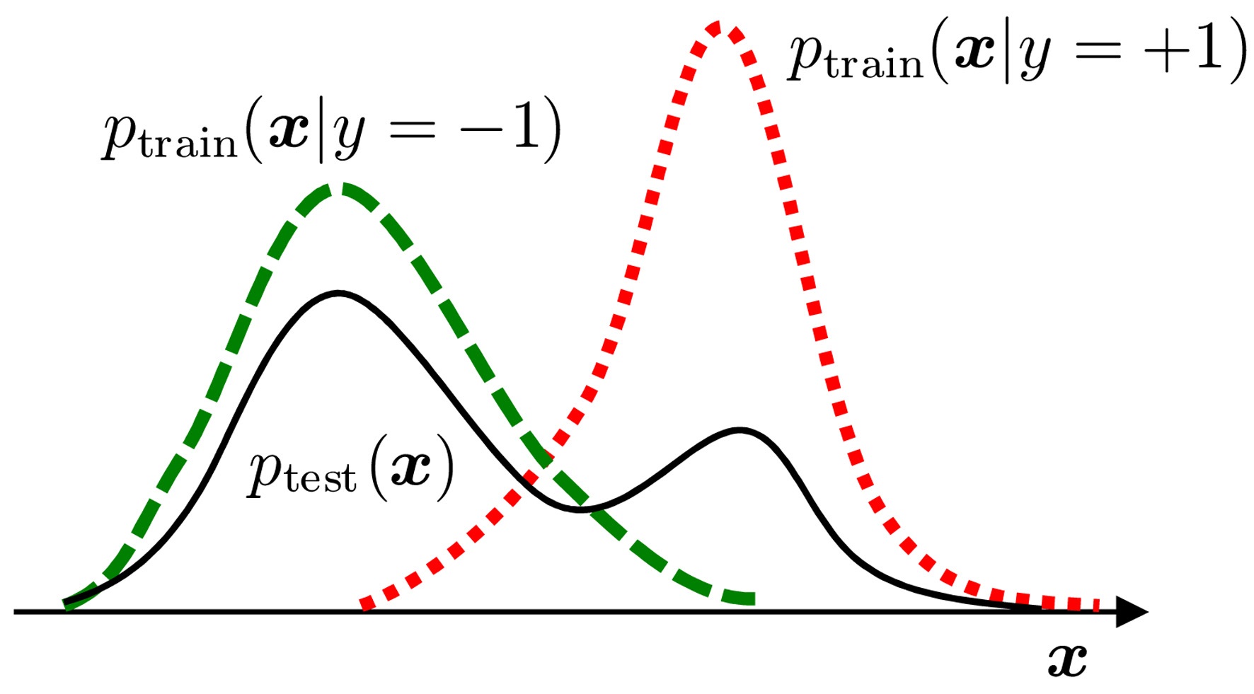
In real-world pattern recognition tasks, changes in class balance are often observed between the training and test phases. In such cases, naive classifier training produces significant estimation bias, because the class balance in the training dataset does not properly reflect that in the test dataset. Here, let us consider a binary pattern recognition task of classifying pattern
The class balance in the test set can be estimated by matching a π-mixture of class-wise training input densities,
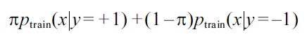
to the test input density
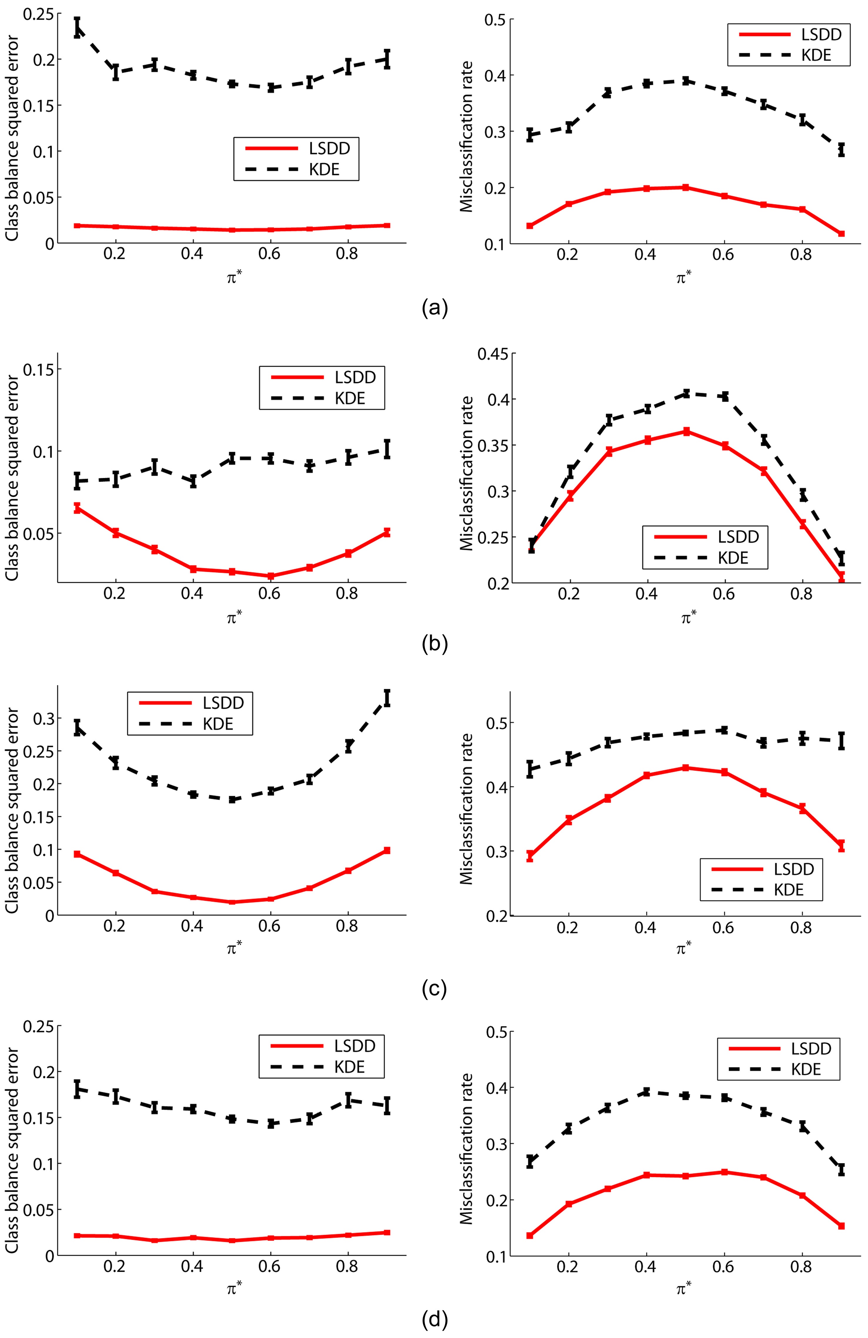
We use four
π* = 0.1, 0.2, ... , 0.9.
The graphs on the left-hand side of Fig. 2 plot the mean and standard error of the squared difference between true and estimated class-balances π. These graphs show that LSDD tends to provide better class-balance estimates than the two-step procedure of first estimating probability densities by kernel density estimation (KDE) and then learning π.
The graphs on the right-hand side of Fig. 2 plot the test misclassification error obtained by a weighted
>
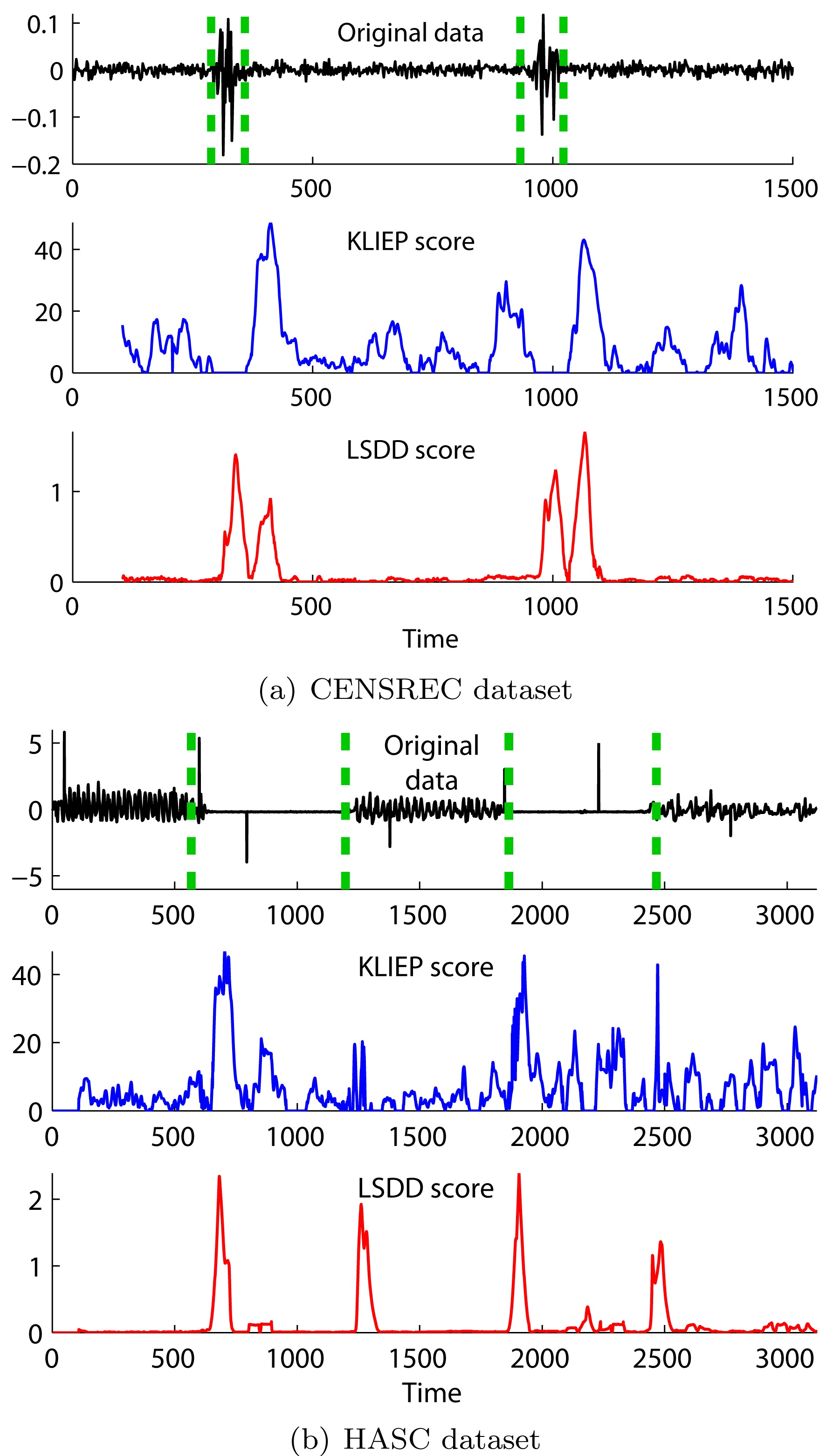
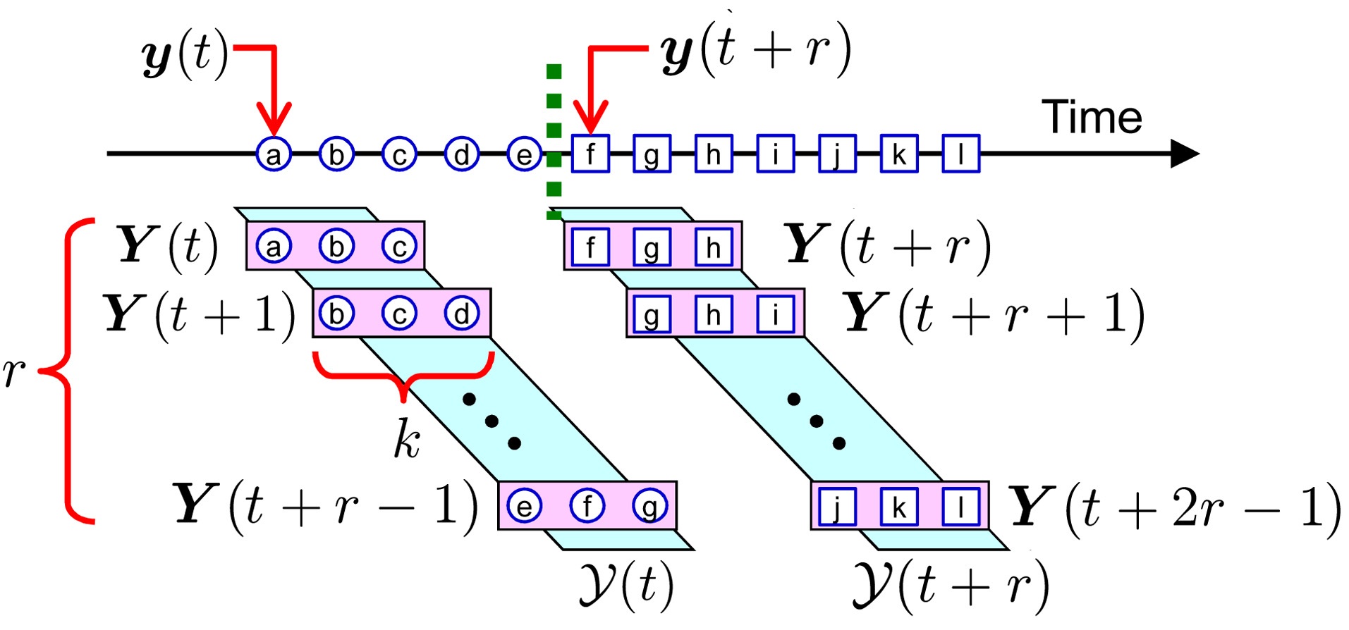
B. Change-Detection in Time-Series
The goal is to discover abrupt property changes behind time-series data. Let
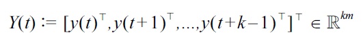
be a subsequence of time series at time
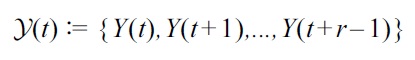
be a set of
In Fig. 4, we illustrate results of unsupervised change detection for the
It was also demonstrated that divergence-based changedetection methods are useful in event detection from movies [6], and Twitter [7].
>
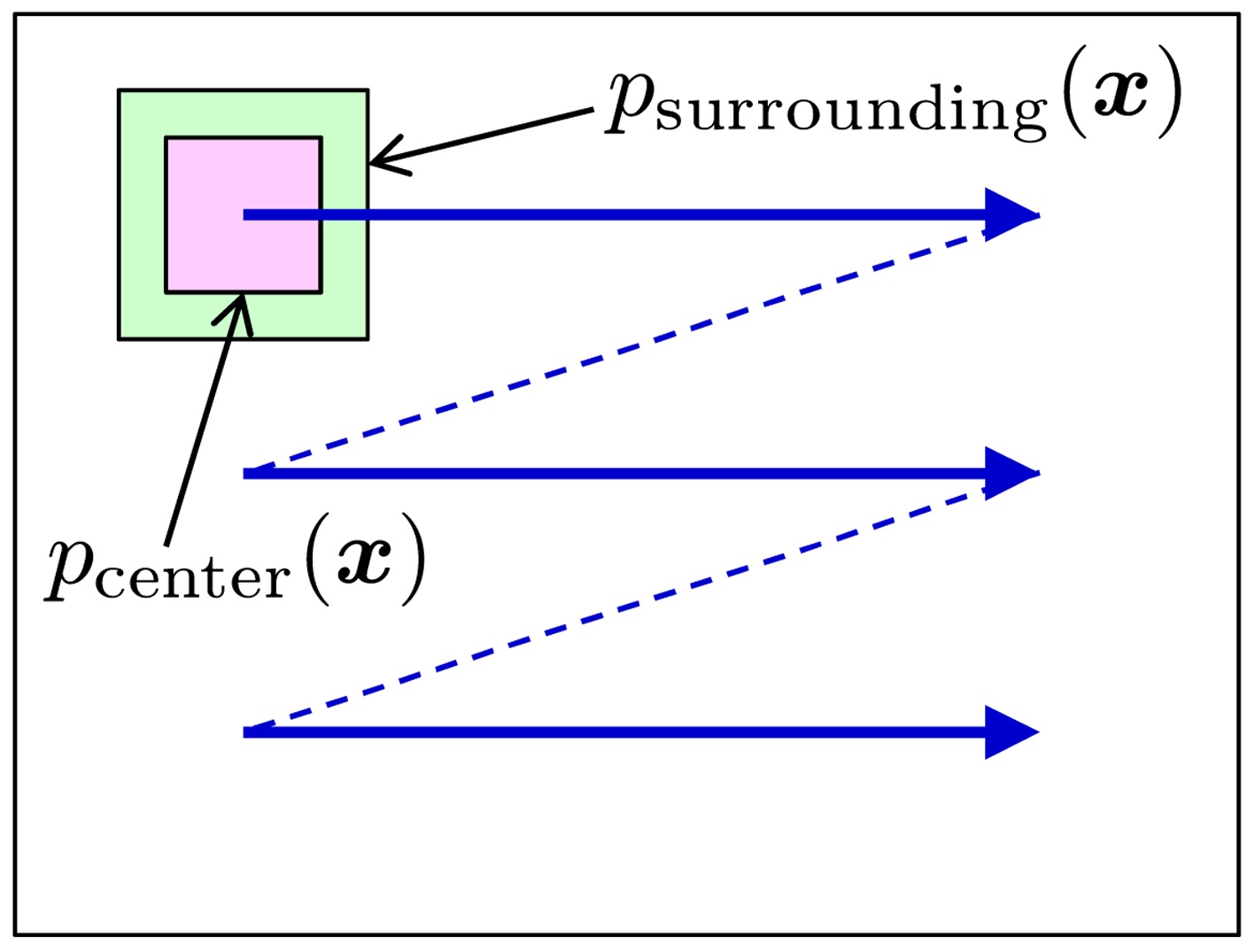
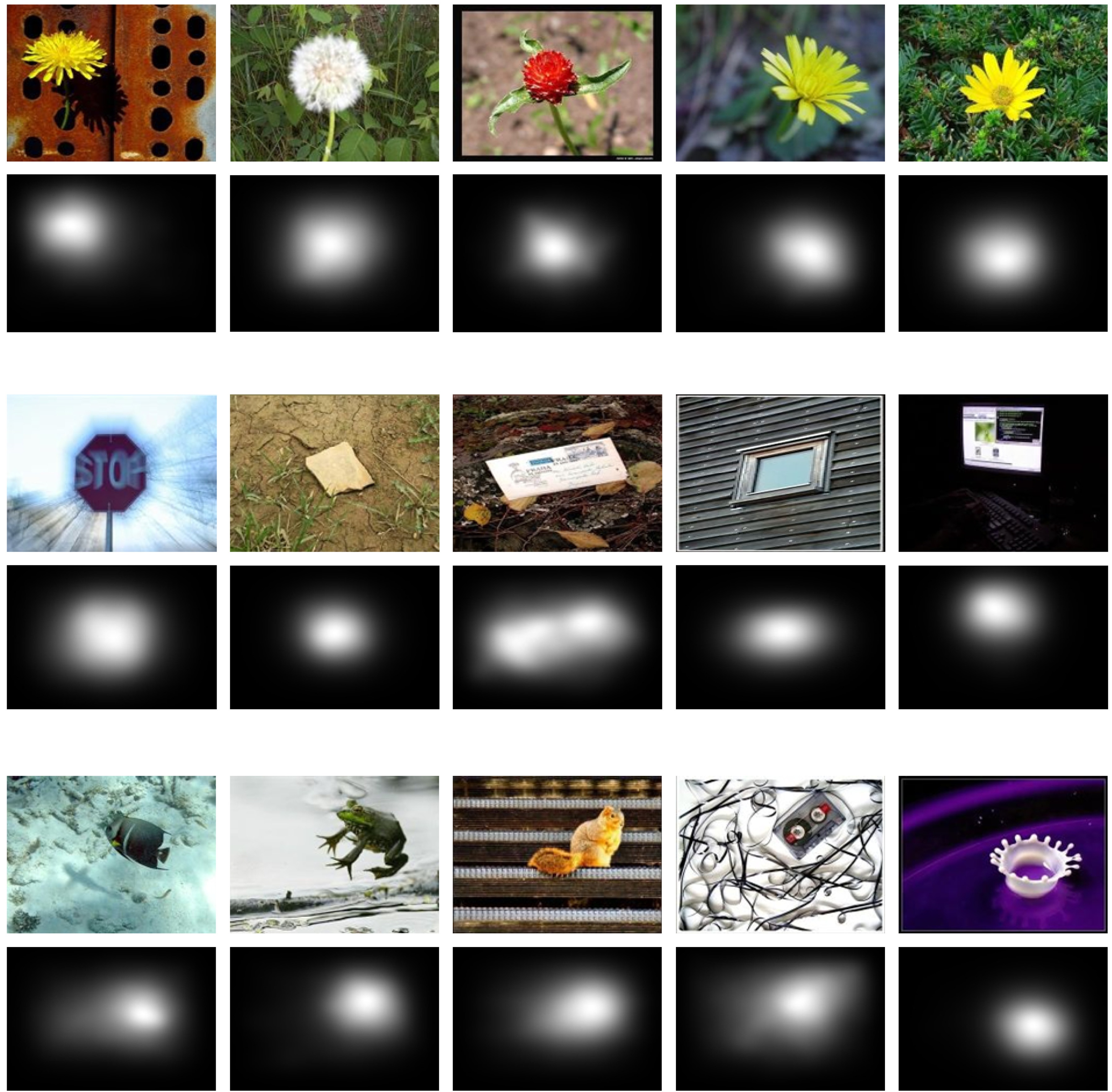
C. Salient Object Detection in an Image
The goal is to find salient objects in an image. This can be achieved by computing a divergence between the prob-
ability distributions of image features (such as brightness, edges, and colors) in the center window and its surroundings [5]. This divergence computation is swept over the entire image, with changing scales (Fig. 5).
The object detection results on the MSRA salient object database [45] by the rPE divergence with
is large. The results show that visually salient objects can be successfully detected by the divergence-based
approach.
>
D. Measuring Statistical Independence
The goal is to measure how strongly two random variables

drawn independently from the joint distribution, with density
Such a dependence measure can be approximated in the same way as ordinary divergences by using the two datasets formed as

The dependence measure based on the KL divergence is called
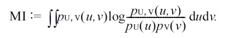
MI plays a central role in information theory [47].
On the other hand, its PE-divergence variant is called the
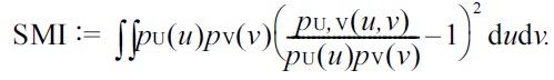
SMI is useful for solving various machine learning tasks [8], including independence testing [9], feature selection [10,11], feature extraction [12,13], canonical dependency analysis [14], object matching [15], independent component analysis [16], clustering [17,18], and causal direction estimation [19].
An
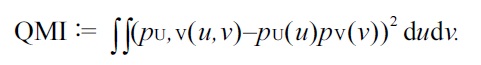
QMI is also a useful dependence measure in practice [49].
In this article, we reviewed recent advances in direct divergence approximation. Direct divergence approximators theoretically achieve optimal convergence rates, both in parametric and non-parametric cases, and experimentally compare favorably with the naive density-estimation counterparts [21-25].
However, direct divergence approximators still suffer from the curse of