In recent brain computer interface (BCI) research, training and calibration times have been drastically reduced due to the use of machine learning and adaptive signal processing techniques [1] as well as novel dry electrodes [2-7]. Initial BCI systems were based on operant conditioning, and could easily require months of training on the subject side before it was possible to use them in an online feedback setting [8,9].
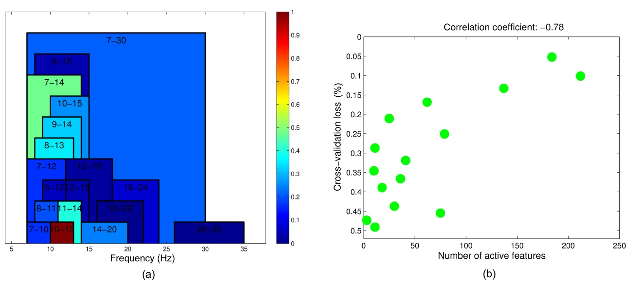
Second-generation BCI systems required the recording of a brief calibration session, during which a subject assumes a fixed number of brain states such as that during movement imagination, after which subject-specific spatio-temporal filters [10] are inferred along with individualized classifiers [1]. The first steps to transfer a BCI user’s filters and classifiers between sessions have been studied [11], and a further online study confirmed that such a transfer is indeed possible without significant performance loss [12]. However, while this work focused on reusing data from previous sessions of expert users, more recent approaches designed subject-independent zerotraining BCI classifiers that enable both experienced and novice BCI subjects to use a BCI system immediately, without the need for recording calibration sessions [13-15]. Various of state-of-the-art learning methods (e.g., SVM, Lasso, etc.) have been applied in order to construct one-size-fits-all classifiers from a vast number of redundant features. The use of sparsifying techniques leads to features within the electroencephalogram (EEG) data that are predictive for future BCI users. The findings show a distribution of different alpha-band features in combination with a number of characteristic common spatial patterns (CSPs) that are highly predictive for most users. Clearly, these type of procedures may also be of use in scientific fields other than BCI, where complex characteristic features need to be homogenized into one overall inference model.
To date, EEG is the most widely used technology in the context of BCI. Some of the main reasons are the relatively low costs and fast setup times partly attributable to the advent of dry-electrode and subject-independent classifiers. Another important reason is the high temporal resolution that EEG offers. However, EEG sensory motor rhythm (SMR)-based BCI still suffers from a number of problems. Unfortunately, not all subjects are able to alter their sensory motor rhythms, and thus, SMR-based BCIs do not work for all subjects. To this end, simultaneous recordings of near-infrared spectroscopy (NIRS) and EEG have not only been shown to increase BCI performance, but have also enabled some subjects to operate a BCI, who previously were not able to do so using solely EEG [16].
While EEG has the highest temporal resolution of all neuroimaging methods, NIRS is dependent on changes of blood flow, as it measures the oxygenated and deoxygenated hemoglobin (HbO2 and HbR) in the superficial layers of the human cortex. The temporal resolution of NIRS is therefore orders of magnitudes lower, which substantially reduces the upper bound of information transfer rates (ITRs) for NIRS-based BCIs. Every neuroimaging method suffers from particular limitations. EEG has poor spatial resolution, while NIRS suffers from sluggishness of the underlying vascular response, which limits its temporal resolution. By employing a multi-modal neuroimaging approach, combining EEG and NIRS, it becomes possible to focus on their individual strengths and to partly overcome these limitations. In particular, we will review how extracting relevant NIRS features to support and complement high-speed EEG-based BCI and thus forming a
II. SUBJECT-INDEPENDENT BCI CLASSIFICATION
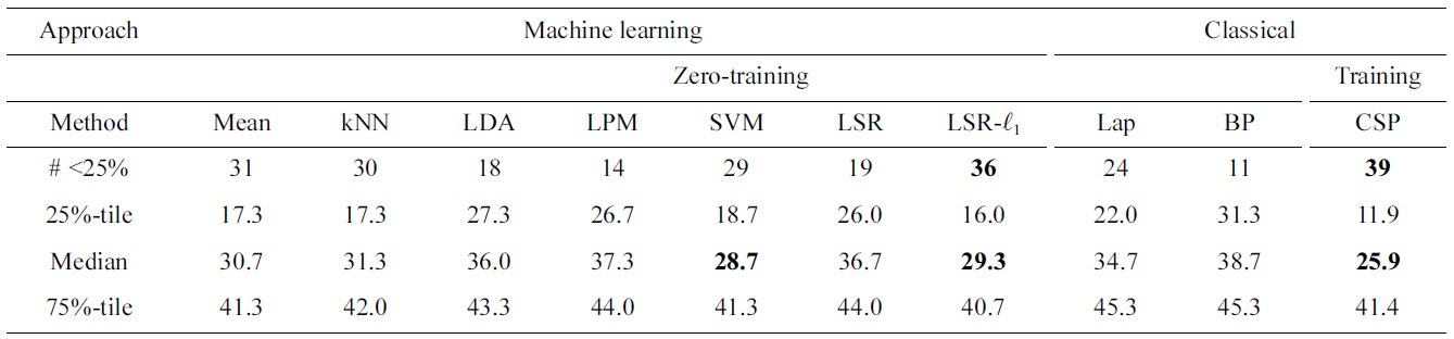
On the path of bringing BCI technology from the lab into practical use, it becomes indispensable to reduce the setup time. While dry electrodes provide a first step to eliminating the time needed for placing a cap, the need for recording calibration sessions has still remained. Employing a large body of high-quality experimental data accumulated over the years now enables the experimenter to choose, by means of machine learning technology, a very sparse set of voting classifiers, which perform as well as the standard, state-of-the-art subject-calibrated methods.
III. MULTI-MODAL RECORDINGS FOR BCI
BCIs that solely rely on NIRS have been realized recently [18,19]. However, when looking at plain NIRS classification rates, it becomes apparent that NIRS cannot be seen as a viable alternative to EEG-based BCIs on its own. However, in a combination with EEG, we find that NIRS is capable of significantly enhancing event-related desynchronization (ERD)-based BCI performance. Not only does it increase performance for most subjects, but it also allows for meaningful classification rates for those who would otherwise not be able to operate a solely EEG-based BCI [16].
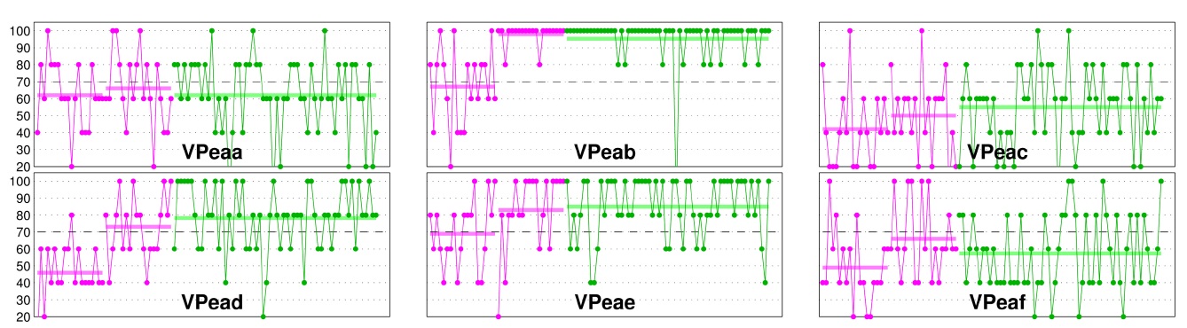
Some subjects, who are able to operate SMR-based BCIs, experience a high level of non-stationarities in their BCI performance, as can be seen in Fig. 2. Possible solutions have been proposed, such as adaptive models [20,21], stationary subspace analysis [22], and a multi-modal approach [23]. The findings indicate that the performance fluctuations of EEG-based BCI control can be predicted by the preceding NIRS activity. These NIRS-based predictions are then employed to generate new, more robust EEG-based BCI classifiers, which enhance classification significantly, while at the same time minimize performance fluctuations and thus increase the general stability

Comparing subject-independent classifier result of various machine learning techniques to various baseline
of BCI performance [23].
Two blocks of real-time EEG-based, visual feedbackcontrolled motor imagery (50 trials per block per condition) were recorded for the estimation of the EEG classifier. The first 2 seconds of each trial began with a black fixation cross, which appeared at the center of the screen. Then, an arrow appeared as a visual cue pointing to the left or right, and the fixation cross started moving for 4 seconds, according to the classifier output. After 4 seconds, the cross disappeared and the screen remained blank for 10.5 ± 1.5 seconds. The online processing was based on the concept of
The user was given instantaneous EEG-based BCI feedback for the two blocks of motor imagery. During the first block of 100 trials, a subject-independent classifier was used, depending on band power estimates of Laplacian- filtered, motor-related EEG channels. For the second block subject-dependent spatial and temporal filters were estimated from the data of the first block and combined with some subject-independent features to form the classifier for the second block. During the online feedback, features were calculated every 40 ms with a sliding window of 750 ms. For further details on
Once the EEG classifier is estimated, a feedback block with 300 trials and a relatively short inter-stimulus interval of 7 seconds is recorded, lasting a total of 35 minutes. As before, the first 2 seconds of each trial began with the appearance of a black fixation cross at the center of the screen. Then, a visual cue in the form of an arrow appeared to indicate the required class, and the fixation cross started moving for 4 seconds, according to the classifier output. After the 4 seconds, the cross disappeared
and the screen remained blank for a short interval of 1 ± 0.5 seconds before the next trial began.
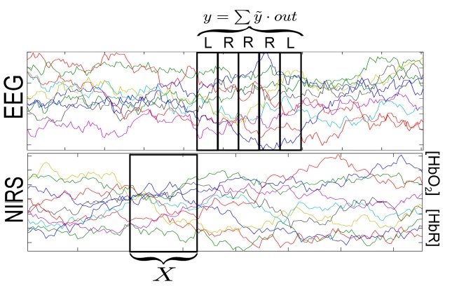
The long inter-trial intervals in the first two blocks were chosen to evaluate the NIRS signals with respect to motor imagery [16]. Here, we only investigate the 300 trials of the fast feedback dataset. These trials are split into chronological blocks of 5 trials each, resulting in 60 blocks and the EEG-BCI performance of these smaller blocks are computed. For each block the EEG-based classifier output,

and summed over the 5 trials within the block, resulting in the performance y of the given block:
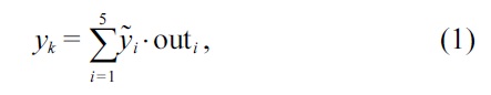
where
The NIRS signal is divided into multiple epochs, each with a width of 2 seconds, preceding each 5-trial block by 2, 4, 6, 8, and 10 seconds. Noisy channels are discarded, and the signal is transferred into the spectral domain. An
where
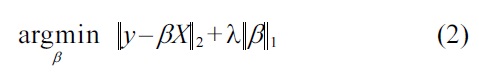
upper part represent trials, where left and right-hand motor imagery are cued. The optimization problem is repeated 60 times, and each time a different block is left out, resulting in a performance prediction for each block. Using the predictions as well as the actual performance, the correlation coefficient and its p-value are calculated. The corresponding p-values test the hypothesis of zero correlation. Since the method is repeated a number of times for various intervals, the p-values are Bonferroni corrected.
Depending on the prediction of the NIRS, the EEG data is grouped into three categories: blocks with good performance, medium performance, and bad performance. All three groups have an even number of trials (100 trials per group). A validation scheme is setup, where one block (consisting of 5 trials) is left out as a test-set. Using the training, set we calculate four EEG classifiers: one for each group, defined by the performance prediction, and a fourth comprising all training data. The individual classifiers

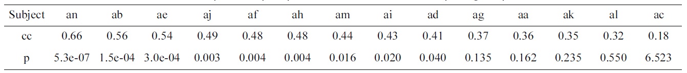
Correlation coefficients (cc) and p-values (p) of predicted vs. actual electroencephalogram performances
[Table 3.] Percentage classification loss of all individual subjects as well as their means
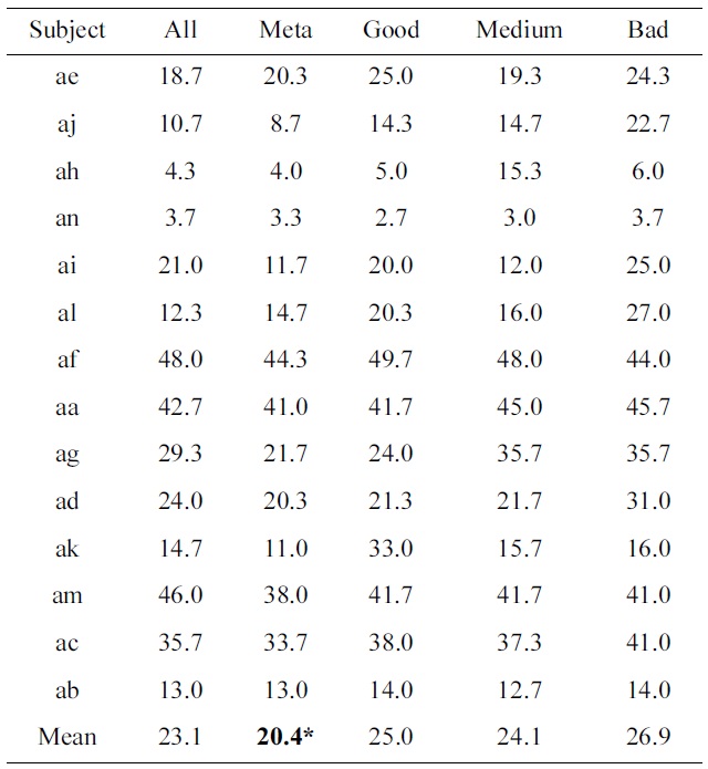
Percentage classification loss of all individual subjects as well as their means
consist of a fixed broadband temporal filter (5thorder Butterworth digital filter with 5?30 Hz), a spatial filter (CSP [10]) and a linear classifier (LDA). In a second step, we train a meta-classifier, combining all four individual classifiers, based on the training set. The outputs of this meta-classifier are then compared to the true labels of the left-out trials, and its 0?1 loss is computed. This procedure is repeated for all blocks. As a baseline, we use the EEG classifier that was trained on all training data.
Table 2 shows the results of the optimization problem defined by Equation (2). For 9 out of 14 subjects, the pvalues of the correlation coefficients calculated between the predicted and actual EEG performance are significant.
Table 3 shows the classification results of all subjects, and their means. A paired t-test between the standard procedure of treating all training trials the same, as compared to a meta-classifier that combines four classifiers, based on the performance of blocks, results in a value of
p = 0.013 (which is indicated by a ‘*’ in Table 3).
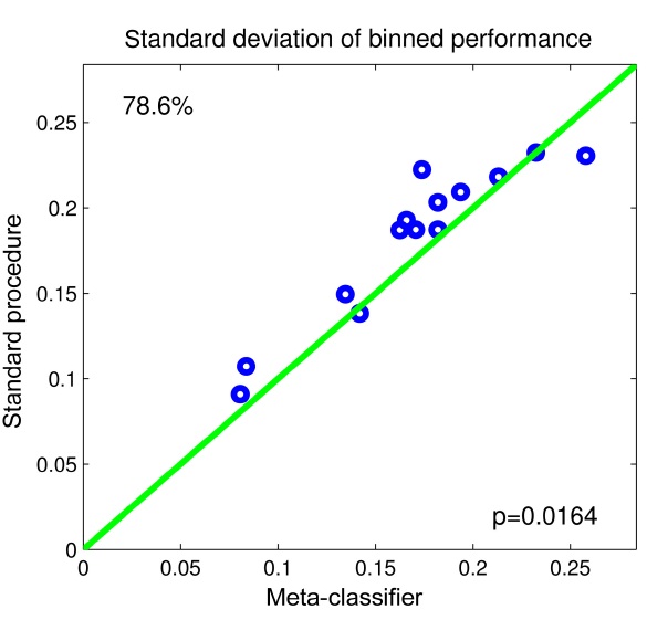
To evaluate whether our method reduces the performance variability during the feedback session, we calculate the standard deviation over all 60 blocks for the standard method, where all trials are treated the same, as well as for the meta-classifier.
Fig. 4 shows the results in the form of a scatter-plot. As can be seen, our proposed method reduces the variability of performance in 11 out of 14 subjects. In one subject, the variability is the same, and for two subjects, the standard procedure has lower performance fluctuations. A paired t-test reveals a significant relationship with p < 0.05.
Multi-modal techniques can be useful in a number of ways. For the case of subject-independent decoding, we found that the outcome of a machine learning experiment can also be viewed as a compact quantitative description of the characteristic variability between individuals in the large subject group. Note that it is not the best subjects that characterize the variance necessary for a subjectindependent algorithm, but the spread over existing physiology is represented concisely.
For the case of combining NIRS and EEG, it can be concluded that this novel approach of combining NIRS and EEG is a viable technique, suitable for SMR-based BCI, since it preserves the responsiveness of the EEG, while at the same time significantly enhances classification rates, and minimizes performance fluctuations.