Brain-computer interfacing (BCI) aims at establishing a novel communication channel between man and machine [1-3]. To this end, brain signals need to be measured noninvasively (electroencephalography [EEG], magnetoencephalography [MEG], functional magnetic resonance imaging [fMRI] or near-infrared spectroscopy [NIRS]), or invasively (multi-unit activity [MUA], electrocorticography [ECoG]). Subsequently, the underlying cognitive states are decoded, and then the user-machine interaction loop is closed by providing real-time feedback about a particular cognitive brain state to the user. From the nonclinical perspective [4], the BCI has also become a very attractive research topic in recent years, since human cognitive states and intentions can be decoded directly at their very origin: the human brain, and not indirectly through behavioral correlates. Note, however, that we should think of the neural correlate as complementary to the behavioral one. A certain cognitive processing might not be visible in the behavioral signal, but may be clearly detected from the neural correlate, e.g., in non-conscious processing [5]. This is particularly interesting in mental state monitoring (e.g., mental workload [6]) or in visual [7,8] and auditory perception tasks [5,9,10]. In this paper, we will report about the latter, as an example of a complex cognitive task, where the decoding of brain states is particularly challenging.
BCI technology has advanced significantly with the advent of robust machine learning techniques [3,11-16] that by now have become a standard in the field. Brain data is characterized by non-stationarity and significant variability, both between trials and between subjects. Oftentimes, signals are high-dimensional, with only relatively few samples available for fitting models to the data, and finally, the signal-to-noise ratio (SNR) is highly unfavorable. In fact, even what is signal and what is noise are typically ill-defined, respectively (cf. [3,11-16]). Due to this variability, machine learning methods have become the tool of choice for the analysis of single-trial brain data. In contrast, classical neurophysiological analysis methods apply averaging methods, such as taking grand averages over trials, subjects and sessions, to get rid of various sources of variability. This approach investigates the average brain, and can answer generic questions of neurophysiological interest, but it is rather blind to the wealth of the dynamics and behavioral variability available only to single-subject, single-trial analysis methods.
In the following, we will focus on behavioral and neural data from the speech signal quality judgements of subjects and their respective neural correlates, as measured by an EEG-BCI. Of particular concern to us is the question of whether or not a participant has behaviorally noticed the loss of quality in a transmitted signal, and whether and how this is reflected in the respective neural correlate. Answering this question is crucial for any provider of signal quality (audio or visual), in order to find the right balance between customer satisfaction and profitability. However, the behavioral ratings of stimuli given by participants are particularly spurious, since the loss of quality is oftentimes at the threshold of perception, so that the participants’ assessments can be unreliable or even close to random guessing. In other words, the label data resulting from such studies lack ground truth. Thus, the label noise is not independent, but―at a perceptual level―it consists of a mix of random labels, and only a few informative ones, and there is no way to tell which is which. This systematic label noise makes the decoding of the respective cognitive brain state hard. So the challenge in our experiment is to decipher, despite a high level of dependent label noise, whether or not the participant has processed a loss of quality on a neural level.
Previous attempts to solve this question (using EEG data for assessing quality perception) employed fully
In the following, we will first introduce the paradigm of the EEG experiment, and explain why the conventional approach is biased. In the third section, we present our supervised-unsupervised learning approach that aims at inferring the correct (neural) labels. The results are presented in the fourth section, followed by a discussion.
II. EEG EXPERIMENT & CLASSICAL ANALYSIS
Understanding which levels of quality loss are still perceived by users is a crucial question for any provider of signal quality. Conventionally, behavioral tests are used for this purpose, asking participants directly for their rating. Recent work has proposed to complement this approach by also recording a user’s neural response to a stimulus, as the neural response may differ from the behavioral response [7,8,17].
Eleven participants (mean age 25 years) took part in this study, for whom both behavioral and neural response were recorded using 64-channel EEG. Participants performed an auditory discrimination task, in which they
had to press a button whenever they detected an auditory stimulus of degraded quality (target). Stimuli were presented in an oddball paradigm, using the undisturbed phoneme /a/ as non-target (NT, 70% of stimuli). Among these stimuli of high quality, the participant had to find instances when the phoneme was superimposed with signal- correlated noise. Participants were instructed to indicate by button press, if they noticed a deviation in the stimulus. Four noisy target stimuli were used, T1-T4, consisting of the phoneme /a/ superimposed with decreasing levels of signal-correlated noise (targets, 6% per class). In an additional 6% of trials, the phoneme /i/ was presented as control stimulus (C, target). The noise levels of the target stimuli (T1-T4) were chosen separately for each participant, in order to account for individual differences in sensitivity to noise, aiming at perception rates of 100%, 75%, 25%, and 0%, respectively. For this purpose, a pretest was run; the resulting SNRs for the deviant stimuli were set to 5, 21, 24, and 28 dB on average (mean perception rate in the experiment: 99%, 46%, 22%, and 7%). The disturbed auditory stimuli were created using a modulated noise reference unit (MNRU [18]). Target stimuli that were detected by the participant are referred to as ‘hits’ (true positives), and the others as ‘misses’ (false positives).
Each stimulus had a duration of 160 ms, with 1000 ms stimulus onset asynchrony. Per participant, 8 to 12 blocks were recorded, with 300 stimuli each. A parallel port computer keyboard was employed for recording the button presses of the participants. For stimulus presentation, in-ear headphones by Sennheiser, Germany were used. EEG was recorded using a Brain Products GmbH (Munich, Germany) EEG system, with 64 electrodes (AF3-4, 7-8; FAF1-2; Fz, 3-10; Fp1-2; FFC1-2, 5-8; FT7-10; FCz, 1- 6; CFC5-8; Cz, 3-6; CCP7-8; CP1-2, 5-6; T7-8; TP7-10; P3-4, Pz, 7-8; POz; O1-2 and the right mastoid), and a BrainAmp (Brain Products GmbH) EEG amplifier. Electrodes were placed according to the international 10-10 system. The tip of the nose was chosen as a reference site, and a forehead ground electrode. EEG data were sampled at a rate of 100 Hz. In the following, we investigate event-related potentials (ERPs), i.e., the differential signal between the voltage at a given electrode position and the reference electrode.
>
B. Taking Wrong Labels at Face Value
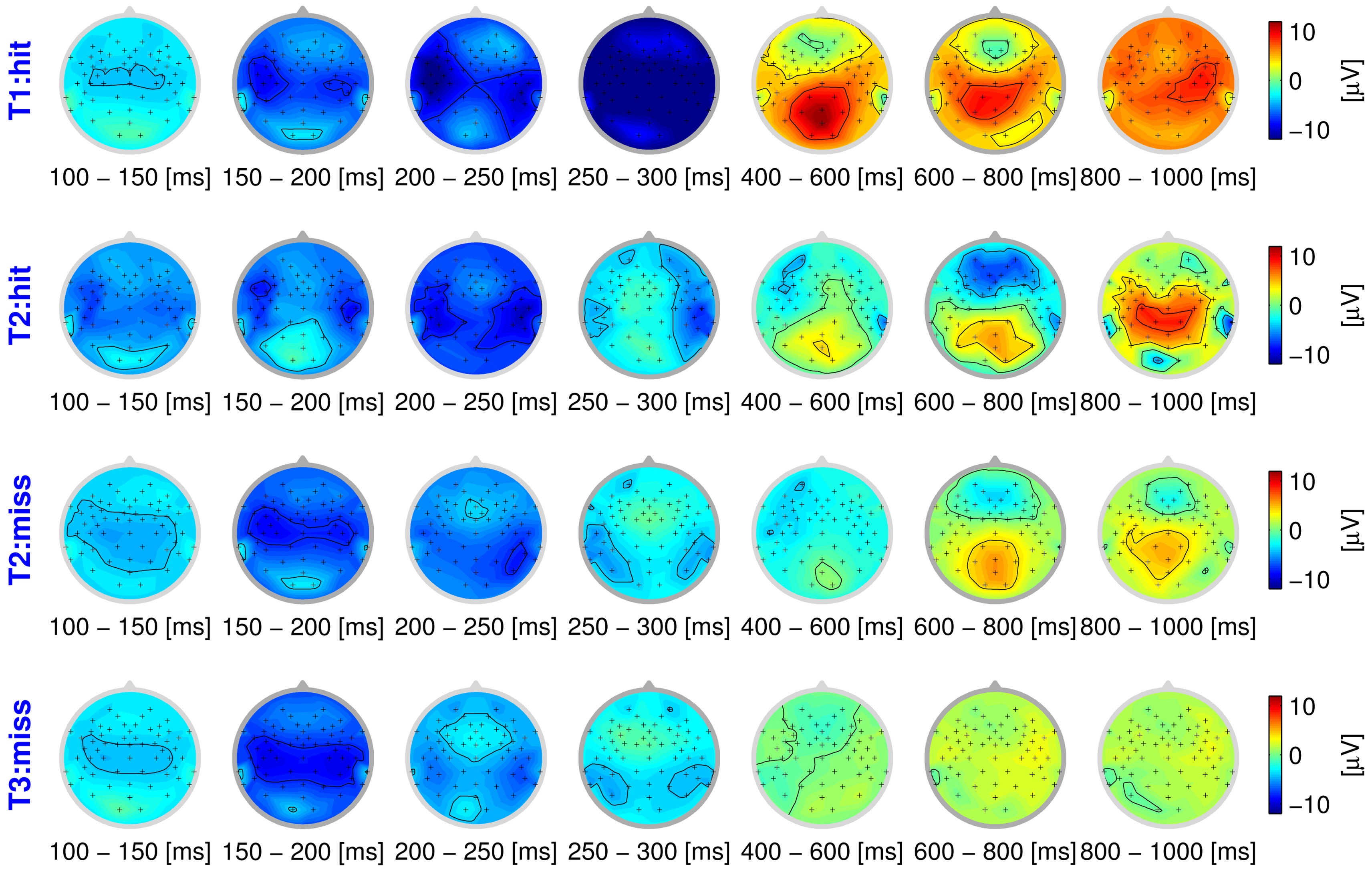
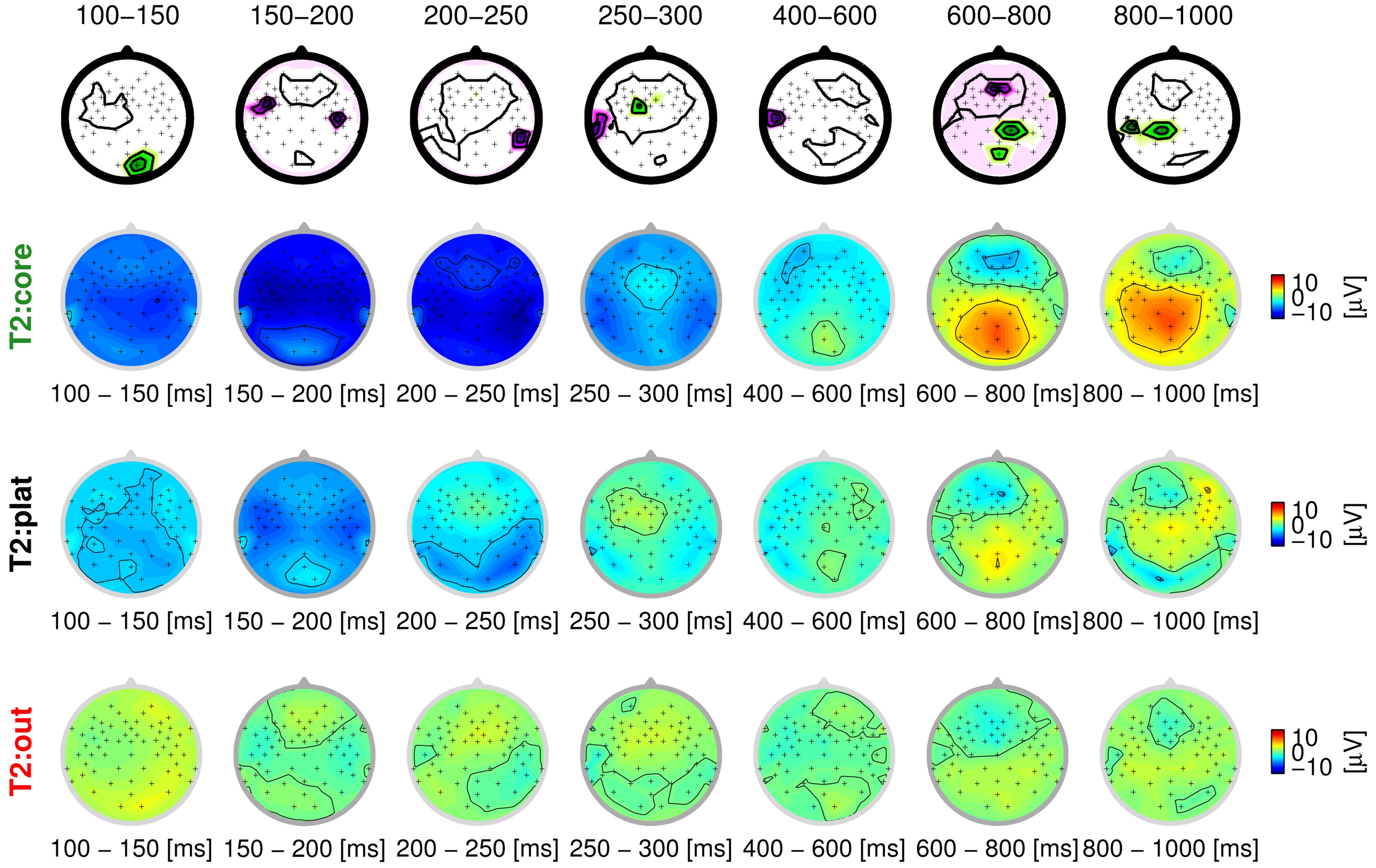
The behavioral responses of the participants provide labels for each trial, seemingly indicating whether the stimulus was perceived as disturbed or not. However, these labels can be assumed to be confounded with label noise to a large degree, in particular at the threshold of perception (stimulus T2). As a first step, we take these spurious labels as ground truth, and analyze the ERPs in these groups. If the behavioral response indicates that the quality degradation is processed (hits), the resulting ERP activation pattern can be characterized by two components: early sensory and late cognitive processing stages. Fig. 1 shows the spatial distribution of the ERPs as scalp distributions (head seen from above, nose pointing upwards), averaged over seven time intervals. The data of one participant (vp = 1) is examined here exemplarily. The top row averaged neural response to a strong degradation that was noticed behaviorally (T1 hit). The four early intervals represent sensory processing of the stimulus (100?300 ms post-stimulus), which is reflected in a temporal negativity above the auditory cortices. In contrast, the last three intervals can be assumed to reflect cognitive processing (400?1000 ms post-stimulus). This elicits an occipital positivity, commonly referred to as P3 component. This component is elicited as a neural reaction to deviating stimuli in an oddball paradigm [19].
In our study, a P3 can be expected to occur when a participant notices that the quality of a stimulus is degraded. Generally speaking, the stronger the degradation, the higher the amplitude of the EEG signal, in particular that of the P3 component. This effect becomes obvious when comparing the first two rows of the figure, with a much weaker activation during late intervals for stimulus T2 (weak degradation), compared to T1 (strong degradation). In contrast, the last row shows the neural processing of a stimulus with a subtle degradation that is not noticed on a behavioral level (T3 miss). While sensory processing still causes activity in the early intervals, there is no notable cognitive component.
While the topography of the averaged ERPs seems to show a consistent picture so far, the presence of label noise becomes very obvious for the stimulus at the threshold of perception (T2). As the ratings of participants become unreliable to the point of guessing, grouping according to behavioral labels becomes conspicuously confounded, as can be seen in the second and third row of
Fig. 1. Even though the participant gave different ratings in these cases, the neural activation is strikingly similar. While the presence of label noise is obvious for this stimulus, the labels of the other classes can be expected to be confounded as well, just to a lesser degree. In the following, we will infer the correct labels in a data-driven way by using a novel learning methodology, in order to obtain an unbiased view of the EEG data.
III. INFERRING THE CORRECT LABELS
Our supervised-unsupervised learning approach aims at finding the true labels based solely on the EEG signal, without taking behavioral labels into account. Technically, we propose a two-step procedure to tackle the dependent label noise problem: (1) outlier detection to remove misleading trials, and (2) a subsequent distinction between labels that are random guesses and the ones that are informative. In the following, we will introduce this novel approach and exemplify it on data from the highly challenging EEG study on speech signal quality assessment, which we introduced in the previous section.
>
A. Abstract Learning Scenario
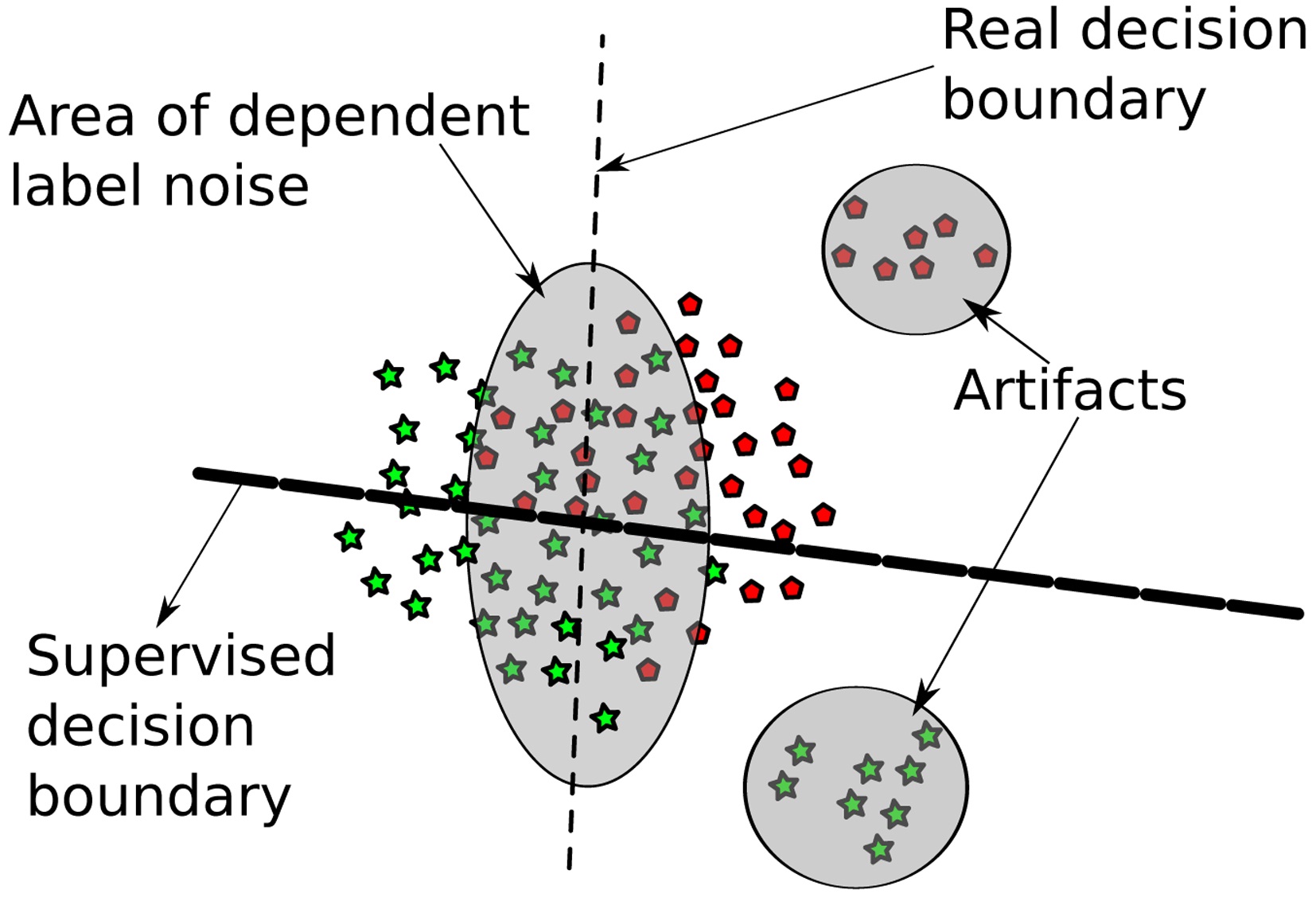
We consider a learning scenario where we have varying confidence in the labels (some are more trustworthy than others). In the considered setup, this stems from two sources: first, some data points are just artifacts, and second, some data points are labeled with very high error rate. The presence of falsely labeled data can hamper learning an accurate decision hyperplane, as illustrated in Fig. 2. Furthermore, some of the settings considered include only a single behavioral class label and hence make supervised learning impossible. As a remedy, we propose a two-step learning approach based on supervised- unsupervised learning, as follows:
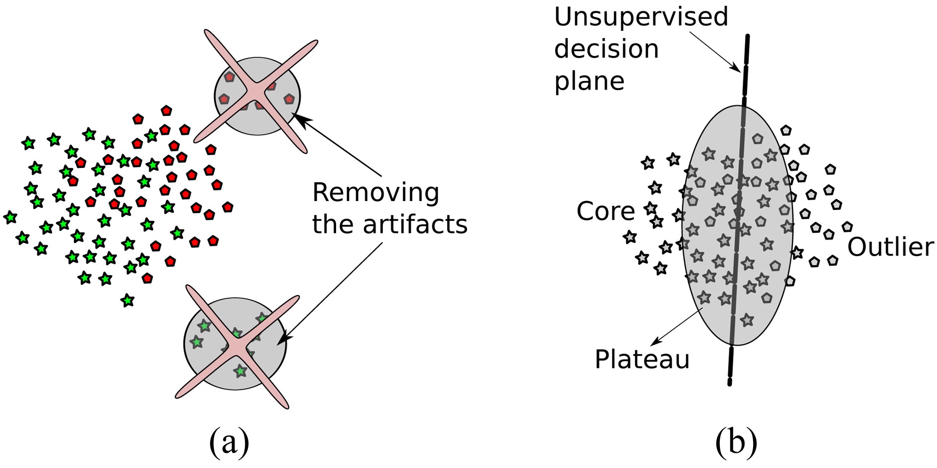
1. Artifact removal: in the first step, as depicted in Fig. 3a, we remove measurement noise, which can in
general stem from broken sensors or, in our case, from faulty electrodes. The steps taken are described in Algorithm 1 lines 1?4.
2. Handling label noise: since we are explicitly not trusting the labels given, in the second step, we train unsupervised on the remaining data points in the second step, resulting in classes that diverge maximal in the data (not necessarily in the labels). The setting is depicted in Fig. 3b, and described in detail in Algorithm 1 lines 6?8.
>
B. Sparsity-Inducing One-Class Learning
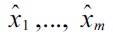
The first step of our approach is based on the paradigms of support vector learning [20-22] and density level set estimation [23]; that is, we are given

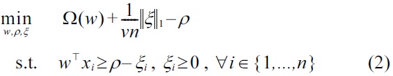
A popular density level set estimator is the so-called one-class SVM [24]
where Ω(
Ω(w) := ?w?p,
where
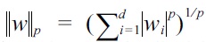
denotes the Minkowski ℓ
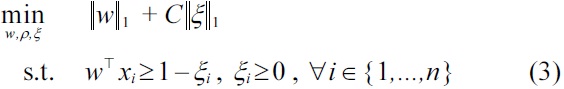
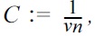
(which is reminiscent of the very well known 2-class CSVM, given by Cortes and Vapnik [25], or sparse Fisher, by Mika et al. [26]). The following theorem shows that Equation (2) is an exact re-formulation of Equation (3). Note that it is sufficient to consider the cases

and
THEOREM 1.
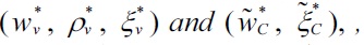
Note that thus

Now denote

By a variable substitution
we observe that
and hence

(because

is the unconstrained version of (3) (and thus equivalent). Thus
For reasons that will become clear later, we wish to also include negatively labeled instances
(i.e., instances of which we already know that they are outliers) into the learning machine (3). A simple and effective way of doing so is to constrain the negatively labeled instances to lie outside of the density level set:

This formulation is a

to lie outside of the density level set
In this section, we describe in detail the proposed supervised-unsupervised processing pipeline. The motivation behind this approach is that, even though it may seem that other methods (e.g., kernelized methods) could be more suitable for this problem, EEG data is well separable by linear classification (for a comparison of linear vs. nonlinear methods, cf. [27]). As discussed previously, the missing ground truth compels us to rely solely on interpretability of the results, which can be achieved easily by applying
The inspection of the results of applying step 1 shows that there is a high chance of finding trials confounded by measurement noise (faulty electrodes) characterized by high amplitudes and/or drifts, which we denote as artifacts. Therefore, we deliberately force the method to exclude such examples and search for other features, by including the highest-ranked data points as outliers in a semi-supervised manner. Typically, we chose five examples of each end of the spectrum, to explicitly retain outlier labels (Algorithm 1 lines 3 and 4).
As illustrated in Fig. 3a, we divide into three classes: core, plateau and outlier class. These classes occur naturally, when applying the sparse one-class methods described in the previous section. Examples belonging to the plateau class are orthogonal to the core and outlier class; these data points lie on the decision boundary. Hence, for division, simple thresholding is sufficient.
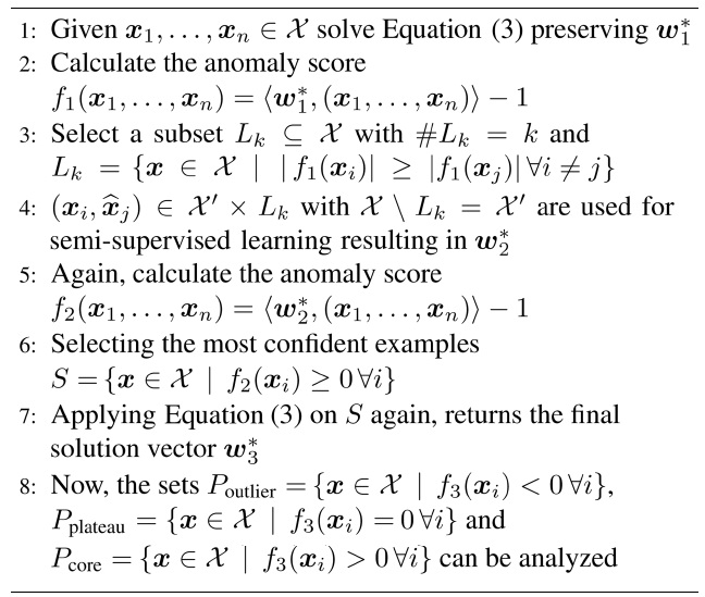
[Algorithm 1] Processing Pipeline

Processing Pipeline
Based on the time series of the ERPs, we first reduced the dimensionality of the data (cf. [12]). Hence, we calculated the mean of the ERP signal within the seven neurophysiologically plausible intervals shown in Fig. 1 (for each electrode and trial). For this, the EEG signal from 61 recorded electrodes was used (omitting the Fp and EO electrodes). Thus, the dimensionality of the data was reduced from 6400 (100 data points × 61 electrodes) to 427 features (7 data points × 61 electrodes). These features were then used as input for the processing pipeline.
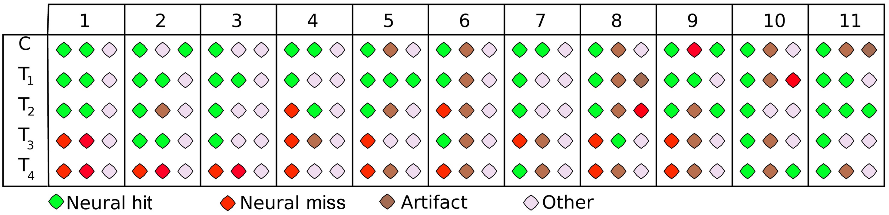
The supervised-unsupervised learning approach groups the trials into three classes: a core class, an outlier class and a plateau class. These three classes can be seen exemplarily in Fig. 4 for one participant (vp = 1) and the stimulus at the threshold of perception (T2). Again, the scalp distribution of ERPs are shown in the seven intervals, which were also used as input features. Remarkably, the core class (row 2) finds a very typical representation of hits with distinct auditory processing (first intervals), and a strong P3 component (last two intervals), suggesting that the degradation was processed consciously. This pattern is subdued in the plateau class (row 3), where the auditory cortices still show a strong activation, but only a very subtle P3 is visible, indicating that the degradation was processed on a sensory level, but not noticed by the participant. Finally, there is virtually no activation in early or late components for the outlier class (row 4), suggesting, at most, subliminal processing of the stimulus. This distinction is more cogent by far than that based on behavioral labels, where two classes were assumed (hit/miss) that were obviously confounded (middle rows of Fig. 1). Not only does the algorithm find plausible classes, it also does so on the basis of neurophysiologically plausible features: as can be seen in the top row of the Fig. 4, the active features reflect the bi-temporal neural activity in early processing stages (auditory) and the occipital activity in late processing stages (cognitive). Across all participants and stimuli, the trials grouped into the core class show a distinct representation of how the stimulus is processed, including both sensory and cognitive components (‘neural hit’) or only sensory processing (‘neural miss’). For obvious degradations (C, T1), it is always the ‘neural hit’ that is found, while the algorithm rather assigns ‘neural misses’ to this class for subtle degradations. This is reasonable; as neural misses can be assumed to be predominant in those classes (the same is true for hits). In almost all cases (participants/stimuli), the outlier class represents trials that reflect a mental state other than these clear hit/miss patterns. Mostly, these are trials with very subdued activation (60% of trials show an amplitude lower
than +/-5 μV on average), which indicates that the stimulus was processed at a subliminal level, at most. Finally, the plateau class, where the EEG signal is orthogonal to the features chosen by the algorithm, contains a cluster of trials that differ most widely among participants. These either reflect measurement noise or eye artifacts (40%), a subdued pattern of neural hits/misses (30%), or a mental state other than that (20%). Fig. 5 summarizes these results, based on visual inspection.
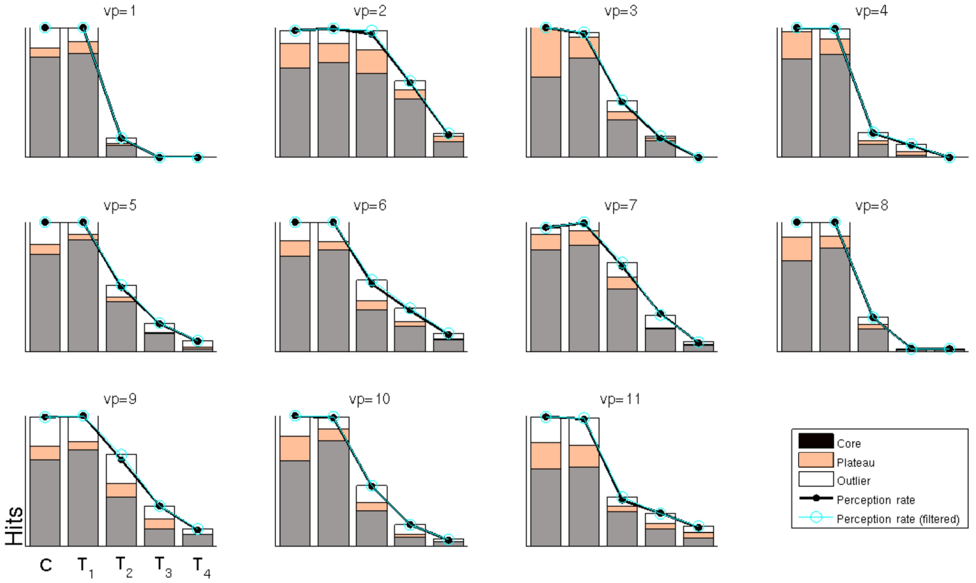
The motivation behind our approach is to find a coherent way to handle dependent label noise that is composed of a mixture of random labels and accurate ones. Fig. 6 provides an insight into these ratios, as far as our approach can reveal them. The behavioral perception rate is shown in black, i.e., the percentage of trials that were labeled as hits by the participants. As can be seen, the perception rate is high (almost 100%) for stimuli C/T1 and then drops markedly for stimuli T2?T4 (left to right). Underneath these values, the figure shows which percentage of these behavioral hits is assigned to the core, plateau or outlier class (ratios shown in gray, orange and white). This could be interpreted as the quantitative mixture of random labels and accurate ones.
Robustly analyzing EEG signals, despite their high nonstationarity (cf. [2,28-30]), their multimodal nature, and the obviously noisy signal characteristics [2], is a major challenge that necessitates machine learning. However, in complex cognitive tasks in particular, the behavioral ratings given by participants are often unreliable, thus introducing label noise. Although in practice, independent
label noise can be handled by most vanilla supervised learning algorithms, they can fail miserably in the case of
Future work will apply our method in the calibration phase of a BCI experiment, where subjects are asked to assume predefined brain states. Here, it is well-known that subjects occasionally do not comply with the instruction given [31] or do not maintain a certain cognitive state throughout the prescribed duration of a stimulus. Our algorithm could thus again contribute to a cleaning of the labels and thus to an increased robustness of the trained BCI system.