Disturbance to plant communities alters the species composition of the stands (Connell 1978, Petraitis et al. 1989). Stands without artificial disturbance would flourish in succession. However, it is difficult to conduct a vegetation survey in a stand without artificial disturbance. Assuming that ideal succession would proceed under circumstances without artificial disturbance, Numata (1961, 1969) proposed a degree of succession (DS) to quantitatively evaluate how plant succession would proceed. He studied the quantitative evaluation of the dynamic process of plant stands based on the life-history traits of constituent species, because he believed that differences among the life-history traits of constituent species would drive stand succession.
Numata (1962) applied his idea to propose an index of grassland conditions to diagnose the degree of grazing in grasslands. Subsequently, Nakamura et al. (2000) applied this idea and proposed a stand quality index to quantify the degree of disturbance caused by over-grazing in the grasslands of Inner Mongolia. However, when Numata (1961) gave scores to species based on the classification of their life-history traits, the number of his categories was only four: annual herb, perennial herb, shrub, and tree. Therefore, using the DS, we were not able to quantitatively separate minute differences between grassland stands with and without disturbances such as prescribed burning in the same stages. Moreover, it was difficult to discern small differences in the length of the restoration period since the prescribed burning.
Here, we propose a more detailed system for classifying the life-history traits of species that grow in Kirigamine semi-natural grasslands. Consequently, we were able to separate minute differences among the stands, thereby quantifying the status of grasslands. Our category system esis based on field experiments of secondary succession conducted by Hayashi (1977, 1992, 2003).
Hayashi concluded that an ideal succession consists of eight stages. When succession proceeds, the dominant species may subsequently be altered. Therefore, the number of alternations of the dominant species until climax is eight. He uses the word “stage” as follows. Following the initial denuding of the plot, the first dominant species gradually appears (the first stage). As succession proceeds, the first dominant species is gradually replaced by a second dominant species (the second stage). The third, fourth, fifth, sixth, seventh, and eighth species become dominant subsequently (the third, fourth, fifth, sixth, seventh and eighth stage, respectively). He predicted the years Y(
We assigned a score to each species as follows. First, we ascertained the life-history traits of the relevant species. Second, we assigned these species to the appropriate stage after considering the coincidence of life-history traits. Third, we assigned a score to each species. This score is the value equivalent to Y(
To assign scores, we must determine the stages of succession to which the species belong. In this report, we determined the life-history traits of species by field observation and references. Consequently, we were able to reduce years of work related to determining the life-history traits of each species through our experiments. Therefore, we have been able to classify species in the stand into the eight stages of succession to assign scores.
The study site was on a gradual slope that was at least 1000 ha in width (Kurihara et al. 2002). The landscape was grasslands with
The mean annual temperature is 6.5℃ and the mean annual precipitation is 1281 mm. Kira’s warmth index is 52℃·month and the cold index is -41℃·month (KiNOA 2012). The soil is black humic soil originating from volcanic ash (Suzuki, personal communication).
>
Treatments of study plots and methods
The study plots consisted of five plots: A, B, C, D, and E. Study plots A, B, and C are situated within 1 km of each other. Study plot D is situated about 4 km east of Study plot C and Study plot E is about 4 km south of Study plot B. Study plots A, B, C, and D are situated at ca. 1600 m a.s.l. The local government of Suwa City and the landowners managed the times and places of the prescribed burning and tree cutting in Study plots A, B, and C. They conducted prescribed burning in spring 2005, 2006, 2007, and 2012 in Study plot A, which is ca. 7 ha wide. In 2012, we conducted vegetation surveys of the quadrats of Study plot A at the end of June (Subplot A1), July (Subplot A2), August (Subplot A3), and September (Subplot A4). Study plot B is ca. 12 ha wide. We divided Study plot B into Subplots B1 (ca. 6 ha) and B2 (ca. 6 ha), because the government and landowners conducted prescribed burning in Subplot B1 in spring 2008 and tree cutting in Subplot B2 in autumn 2008. Study plot C was ca. 6 ha wide and they conducted prescribed burning there in spring 2009. Study plot D consisted of Subplots D1 (ca. 2 ha), D2 (ca. 2 ha), D3 (ca. 1 ha), and D4 (ca. 2 ha). The landowners of D1 conducted prescribed burning in Subplot D1 in the spring of every year. Ski companies governed Subplots D2 and D3, so they conducted mowing without removing the mowed grass in Subplot D2 in the autumn of every year and tree cutting without removing the cut trees in Subplot D3 in the autumn of every year. We left Subplot D4 without treatment from 1967 to autumn 2012. In Study plot E, situated at ca. 1300 m a.s.l.,
In each subplot, we arbitrarily placed 1 m × 1 m quadrats so that the distance between the quadrats was greater that 5 m (Okutomi and Itow 1967). The numbers of quadrats we placed in each subplot were 10 in Subplot A, 12 in Subplot B1, 12 in Subplot B2, 11 in Subplot C, 17 in Subplot D1, 6 in Subplot D2, 4 in Subplot D3, 9 in Subplot D4, 6 in Subplot E1, 6 in Subplot E2, and 6 in Subplot E3. We measured the maximum height (cm) and visually essinentimated the coverage (%) of the quadrats of every species growing in the quadrat and the total coverage (%) of the quadrats. We conducted vegetation surveys of Study plots B, C, D, and E between the end of August and the end of September 2012. On 25 Sep 2012, we clipped the aboveground biomass of the constituent species in a 1 m × 1 m quadrat near Study plot A and dried them for 48 h at 60℃. On 22 and 29 Oct 2012, we measured the population density, height, and crown size of the
>
Definition of index and calculation
To quantify the dynamic status of each subplot, we defined the index of dynamic status (IDS) by

where

The
We determined the
When we determined the stage that the concerned species belong to, we focused on the following life-history traits. Because the species of the first stage of an ideal succession is an annual herb that produces seed of the clitochore type, we focused on the life-history traits of annual herbs and the production of seeds of the clitochore type. Consequently, we classified species with life-history traits of annual herbs and the production of seeds of the clitochore type into species of the first stage of succession. Similarly, species that had life-history traits of biennial herbs and the production of seeds of the anemochore type were classified into the second stage of succession.
Species of the third and fourth stages are both perennial herbs, but those of the third stage have elongated rhizomes and those of the fourth stage form tussocks. Growth form tufts are strongly related with the life-history trait of making tussocks (Shimizu 2001). Consequently, we assigned species with perennial herbs and growth form tufts to the fourth stage. In Nemoto’s study (2006), almost all species of the fourth stage consisted of species with growth form tufts and perennial herbs. Growth form tufts occurred mainly in Poaceae and Cyperaceae (Tsutida and Suganuma 1978, Shimizu 2001).
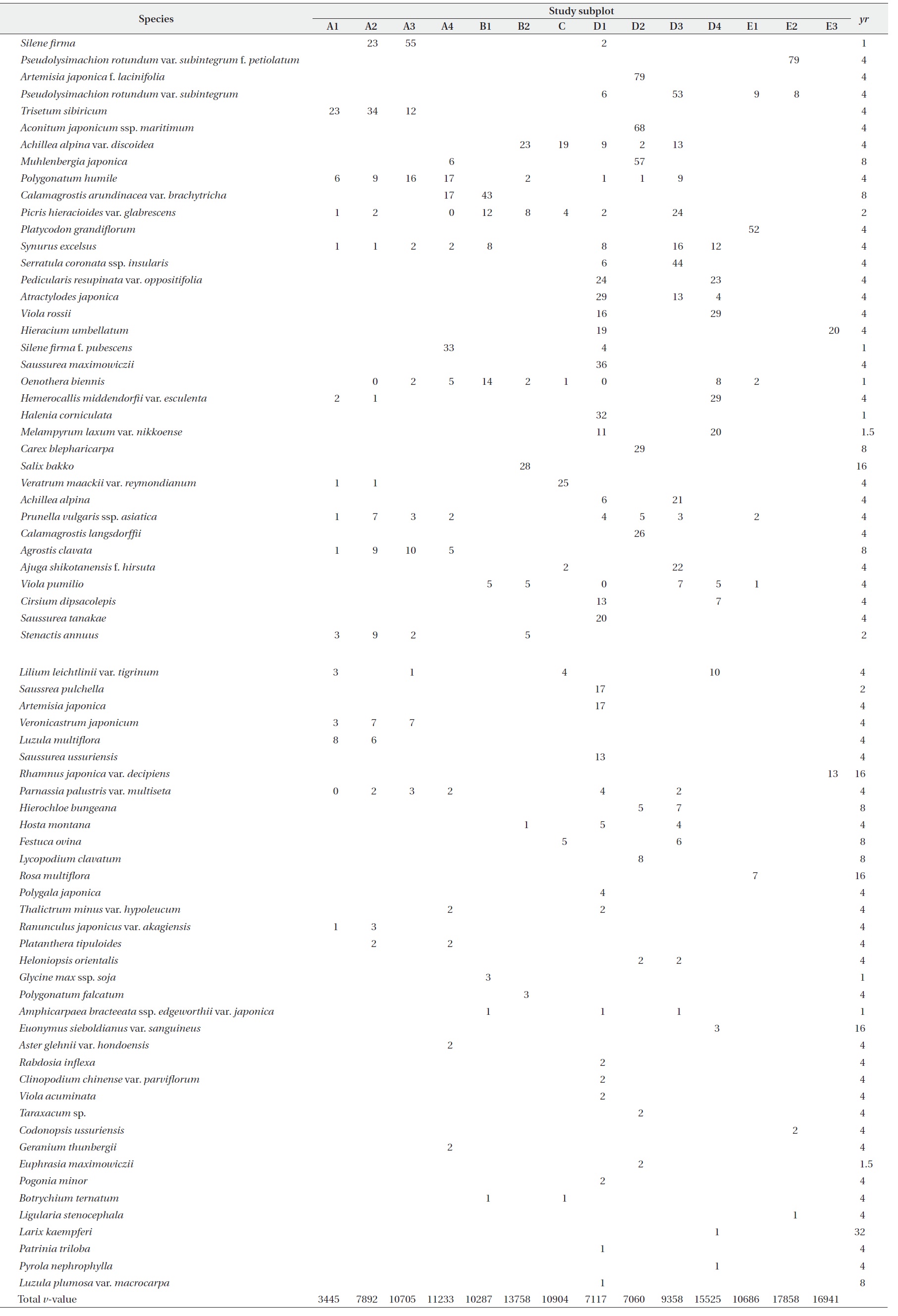
When we determined species life-history traits such as dormancy form, disseminule form, growth form, and flowering period, we referred to Numata and Yoshizawa (1975), Numata (1990), Osada (1993), Shimizu (1997), Asano (2005), and Hoshino and Masaki (2011). We referred to Miyawaki et al. (1994) for dormancy forms N, M, and MM. Some species have multiple growth forms (Numata 1957). Consequently, when we were not able to classify a species into a single stage, we assigned the score of the mean value between the corresponding two (e.g., if it was difficult to classify whether the score of a species was one or two, we gave 1.5).
The relation between
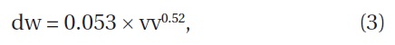
where dw is the above-ground dry weight (g) and vv is the
Species compositions and their
[Table 1.] Species composition and ν-value(102 cm3/m2). See text for yr.
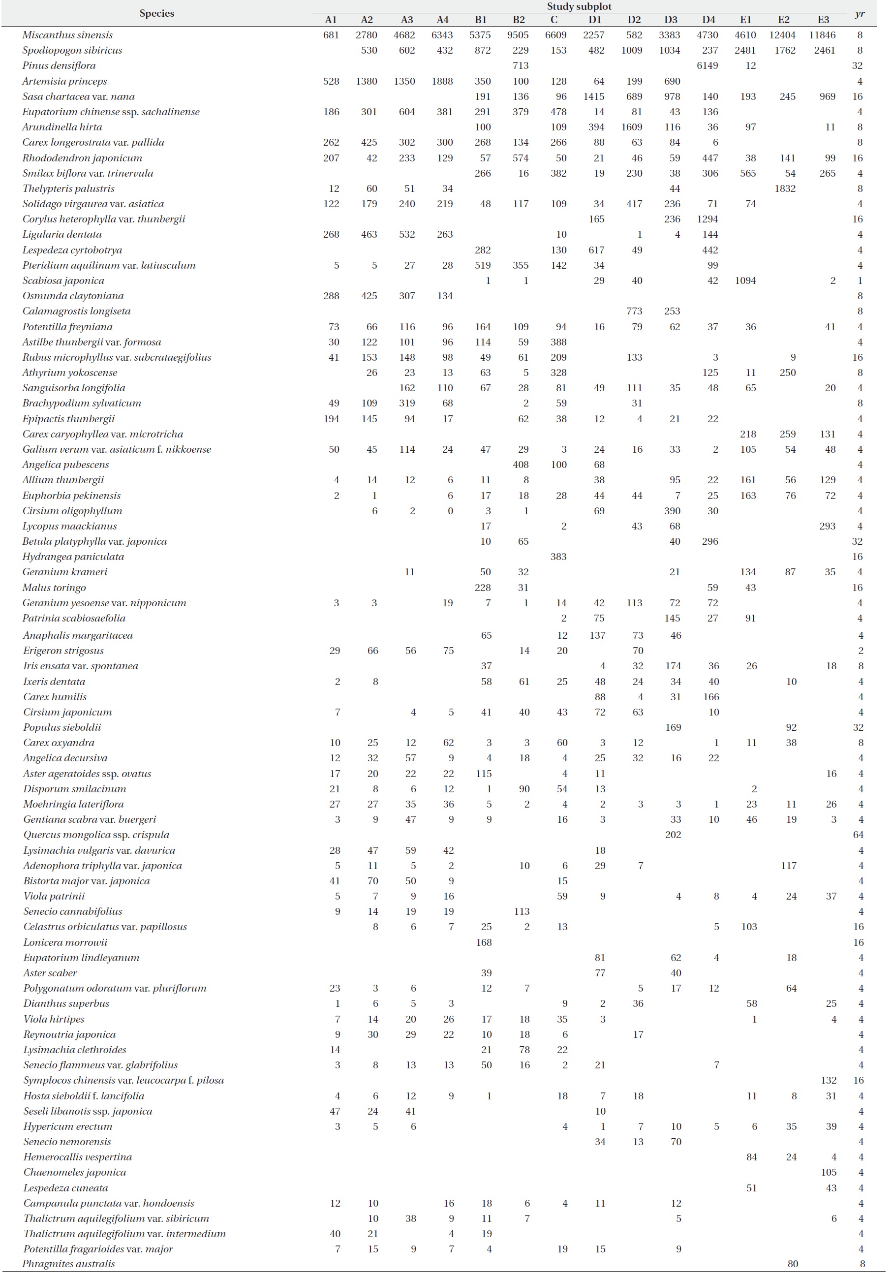
Species composition and ν-value(102 cm3/m2). See text for yr.

Continued
were the largest among the constituent species. The sum of the
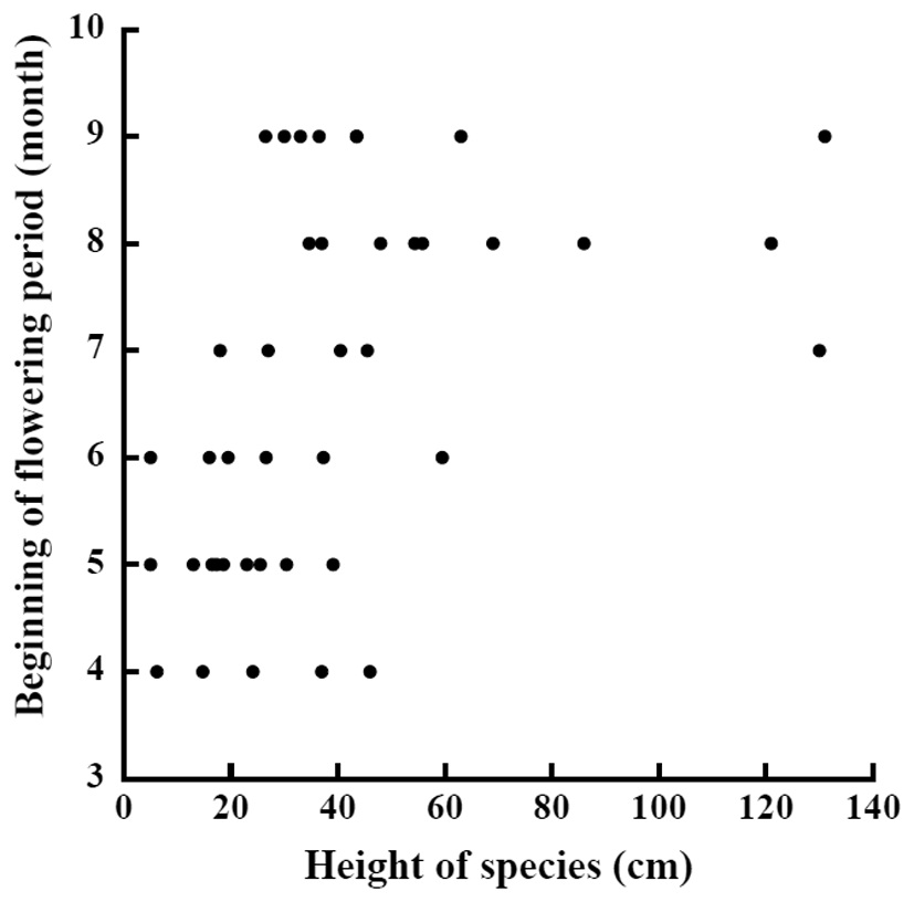
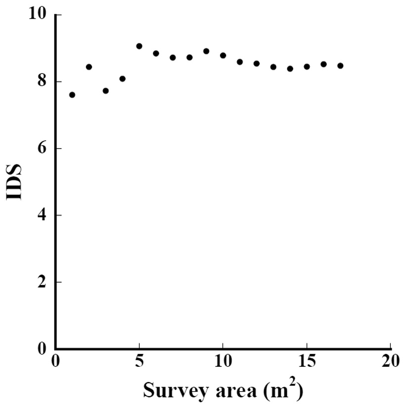
The species-area curve of Subplot D1 is shown in Fig. 2. The total number of species continued increasing in the 17 m2 area. We should survey a wider area to record all growing species.
The relation between the indices and survey area in Subplot D1 is shown in Fig. 3. When the survey area was 17 m2, the IDS was 8.5. Even when the survey area was 1 m2, the IDS was within ±10% of the value 8.5. Furthermore, when the survey area exceeded 6 m2 and 11 m2, IDS converged was within ±5% and ±1%, respectively. The IDS converges into a value at smaller areas than the area needed when the number of species converges.
The IDS in Subplot A1 was 6.4, Subplot A2 was 6.5, Subplot A3 was 6.8, and Subplot A4 was 6.9. We conducted vegetation surveys in Subplot A1 2 months after the prescribed burning, in Subplot A2 3 months after burning, in Subplot A3 4 months after burning, and in Subplot A4 5 months after burning. The indices gradually increased in the growing season. The indices were 7.5 in Subplot B1 and 7.6 in Study plot C. We conducted vegetation surveys in Subplots B1 4 years after prescribed burning and in Study plot C 3 years after burning. The indices were larger than those of plots within a year after the prescribed burning. The IDS of Subplot B2 was 9.2. The IDS was 8.5 in Subplot D1, 7.8 in Subplot D2, 9.7 in Subplot D3, and 18.5 in Subplot D4. The IDS was 6.9 in Subplot E1, 8.1 in Subplot E2, and 8.2 in Subplot E3.
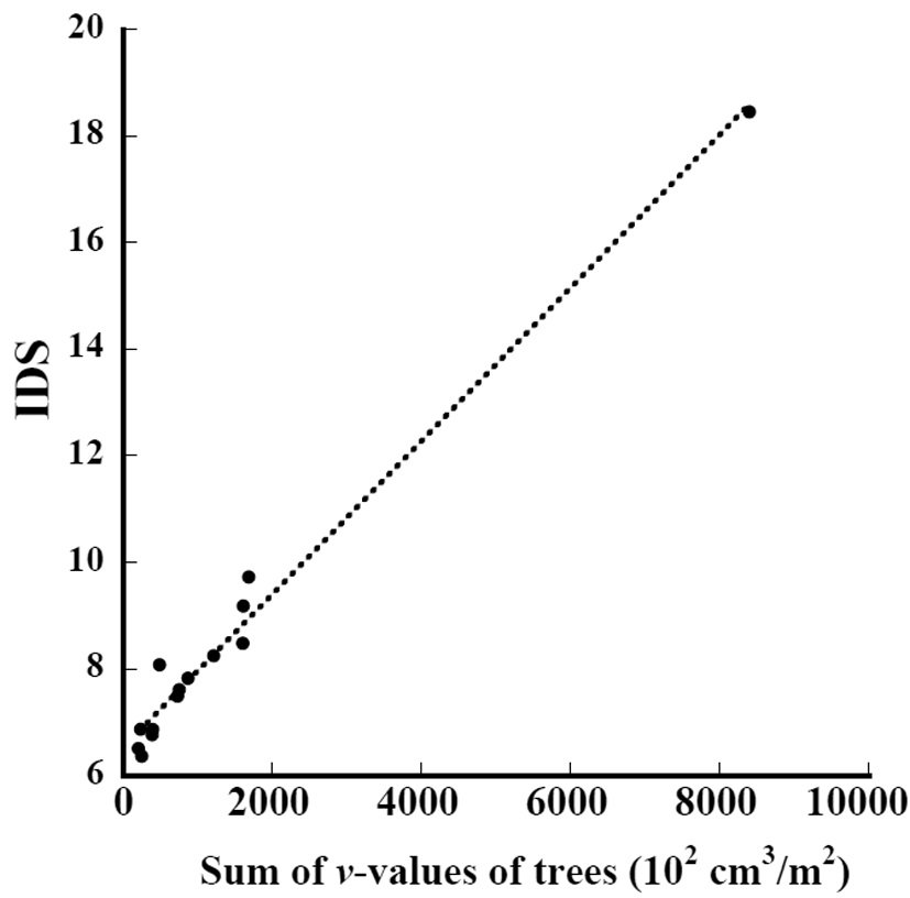
The relation between the sum of the

where IDS_t is the IDS of the subplots in this study and
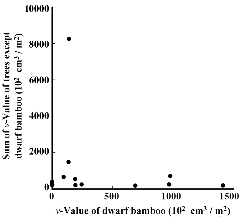
The relation between the
bamboo grew. Among the percentages of
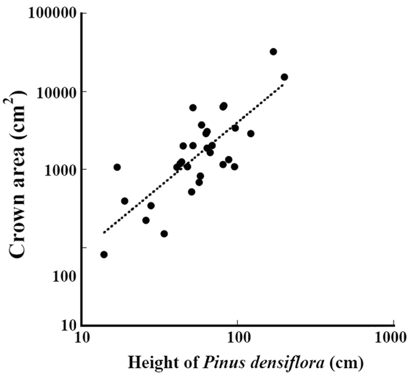
The relation between the height of

where crown_a is the crown area (cm2) and height_p is the height (cm) (Fig. 6) (ANOVA, F1,29=11.5, P = 0.0019). The crown area was significantly correlated with the height.
The number of
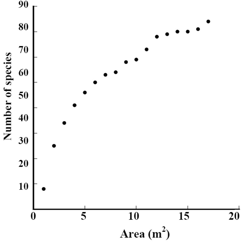
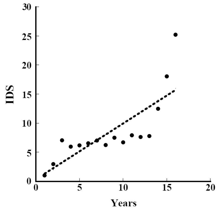
Iijima and Sado (2005) conducted experiments on secondary succession for 16 years after they denuded the area. We calculated the

where IDS_i is the value of the IDS by Iijima and Sago’s data and year_L is the years since they started the experiment from the denuded area (Fig. 8) (ANOVA, F1,14=22.97, P = 0.000286). The indices were significantly correlated with the length of years in secondary succession since they denuded the area. The increment of change in the IDS per year was 0.96.
According to Prach (1990),
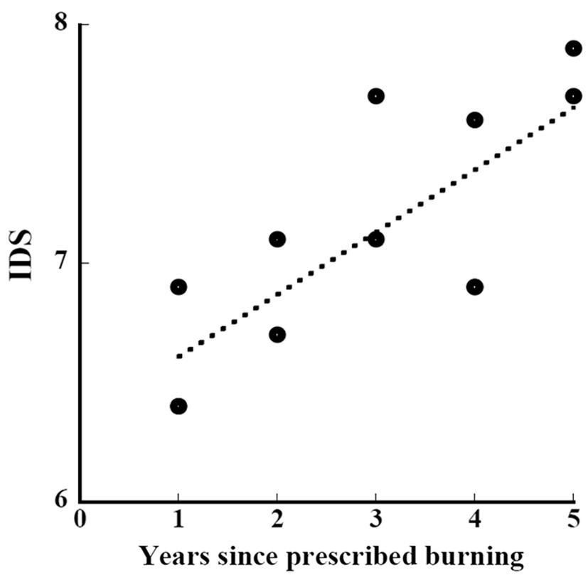
Kawakami et al. (personal communication) conducted vegetation surveys for 4 years between 2008 and 2011 in the same study area as ours and set a total of 179 1 m × 1 m quadrats. We calculated indices using their data of height and coverage. The relation between the length of years of restoration since the prescribed burning and the indices of their study and ours was approximated by
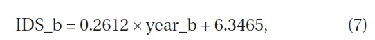
where IDS_b is the IDS of the subplot and year_b is the years since the prescribed burning of the subplot (Fig. 9) (ANOVA, F1,10=14.54, P=0.0034). The indices were significantly correlated with the length of years of restoration. The increment of the IDS in a year during the restoration period since the prescribed burning was 0.26. The increment of 0.26 per year is as small as one-fourth of the aforementioned increment of 0.96 in succession without disturbance.
According to the reports of Negishi and Yagi (1985), Wu and Ando (2008), and Ogura (2009), the relation between the age and the height of the initial growing stage of

where height_pd is the height (cm) of
Because they conducted tree cutting in Subplot B2 in autumn 2008, the ages of
Using Equations (5) and (8), we were able to estimate the volume, the product of the crown area and the height, of
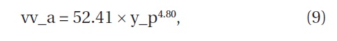
where vv_a is the volume (cm3) of
Furthermore, with a mean annual establishment rate, 0.11 individuals m―2 year―1, we were able to estimate the increment of

where Δvv is the increment of
Of the 14 subplots, the mean of the sum of
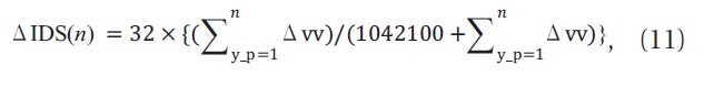
where, Δ IDS(
With Equations (10) and (11), we were able to estimate Δ IDS (5), which is the contribution by
We estimated the IDS of grasslands with the coverage and height of constituent species. Using the IDS, we quantitatively analyzed the effect of the disturbance of prescribed burning. Trees are affected by the disturbance of prescribed burning. We calculated, using the annual establishment and growth rates, the contribution by