In In the field of remote sensing and earth observation utilizing microwave radar systems, the method of moments (MoM) with the Rao-Wilton-Glisson (RWG) basis function and its derivatives is widely used to compute the scattering properties of an arbitrary object [1], [2]. Recently, the use of this numerical analysis technique has been proposed in various studies to analyze the scattering property in half-space, which includes multiple scattering between scattering particles and bottom surfaces [3], [4]. Development of these numerical techniques is very useful in the remote sensing of earth terrain because the scattering process from scatterers randomly placed on a flat surface, such as a water surface or ground plane, can be represented well by a half-space scattering that applies the image theory or the impedance boundary condition [5].
In particular, due to the edges laid on the interface, the placement of a scatterer on an infinite conducting or impedance surface results in complications in computational processes such as singularity or inaccurate calculations by original sources and their images on the same surface. Image theory [6], [7] and a recent study [3] do not consider this contact problem, so some ambiguity exists for numerically solving the scattering property of a flat surface that includes various scatterers. Thus, we effectively solved this issue on the half-space scattering problem using the MoM process with RWG basis function by proposing a virtual vertex technique whereby the contact surface of the scatterer can be removed and replaced by the half-RWG basis of the boundary edge on the interface of half-space and an additionally inserted virtual vertex [4], and we clearly show its angular effect in this study.
Virtual vertices inserted for effective treatment of the problematic boundary edges in half-space scattering can be located essentially at any position of the upper halfspace, including the interface. One of the possible solutions is to place them on the interface of the half-space. In this case, a half-RWG basis vector generated by the virtual vertex has only tangential vector components, which will be canceled by their images when we apply an exact image theory to solve the half-space scattering problem, such as a conducting hemisphere laid on an infinite conducting surface [6], [7].
However, several arguments about the effect of virtual vertexes persist. For example, in the case of a scattering object that includes a scattering surface perpendicular to the ground surface, we usually encounter singular points when the electric field integral equation (EFIE) is used to solve the problem because the projection of orthogonal vectors becomes zero. Therefore, the virtual vertex in this case does not contribute to a computational result and even frequently creates a singularity in the computational procedure [8], [9]. In other words, when the original half-RWG basis vector and the added half- RWG basis by the virtual vertex are perpendicular, the effectiveness of the insertion of a virtual vertex becomes questionable.
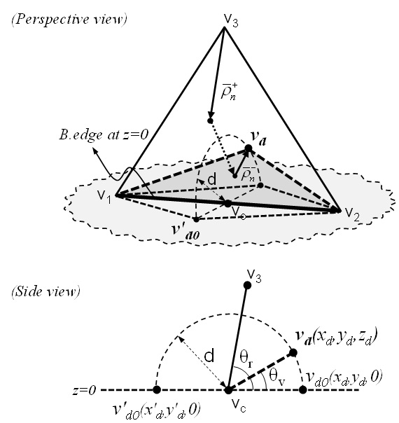
We investigated the effect of the position of a virtual vertex by first introducing a conducting plate whose side (boundary edge) is attached to the ground surface, as shown in Fig. 1, with an inclination angle
In the present study, we discuss the angular effect of virtual vertices. When we apply existing numerical techniques [1], [8], [9] to solve the half-space scattering problem, an optimal position for a virtual vertex will be determined to provide accurate numerical results for scattering from an arbitrary object on a conducting surface. The EFIE was used in the present study to compute these scattering problems with an open-structure, such as a conducting plate.
Ⅱ. Virtual Vertex in Half-Space
The geometrical parameters associated with an arbitrary virtual vertex in the upper half-space and the floating boundary edge on the interface are shown in Fig. 1. Insertion of a virtual vertex results in incorporation of a half RWG basis of the boundary edge into the MoM process to depict the vertical current components passing through it [4], [6], [7]. The angular effect of a virtual vertex in an arbitrary angle is examined by computing the scattering properties of test objects with various angles of
2-1 Modified Electric Field Integral Equation
We computed the scattering property of a test object with various angles using the modified integral equation with the original current sources and their images. The original current sources

and their images

are expressed as shown in (1) and (2) [10].


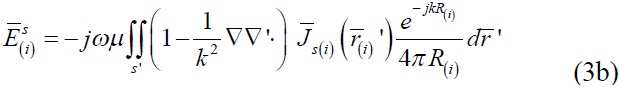
The scattered fields

due to the original and image curent sources can be represented as shown in (3) [4].

where subscript ‘
were computed using numerical integration with Gaussian quadrature over triangle [8] and analytic integration for singularity extraction from self-cells [9]. In particular, this analytic integration may cause another singularity if the observation vector

(a projection of observation vector

) lies anywhere along an edge. In this case, we moved the observation point a very small distance (

where
are position vectors of the original and updated positions for the observation point and
2-2 Test Setup & Virtual Vertex
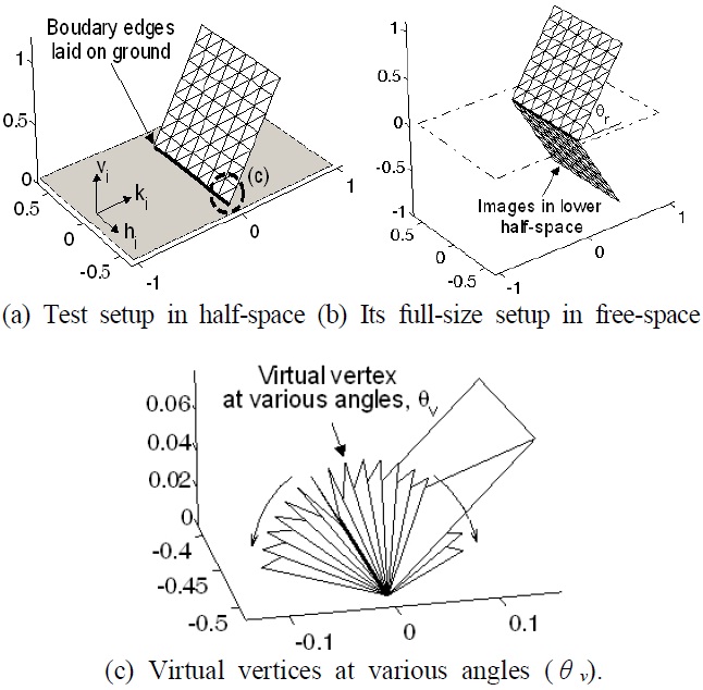
We examined the angular effect of virtual vertices by first computing the RCS of a 1
The starting and ending points of a boundary edge are
2-3 Insertion of Virtual Vertices
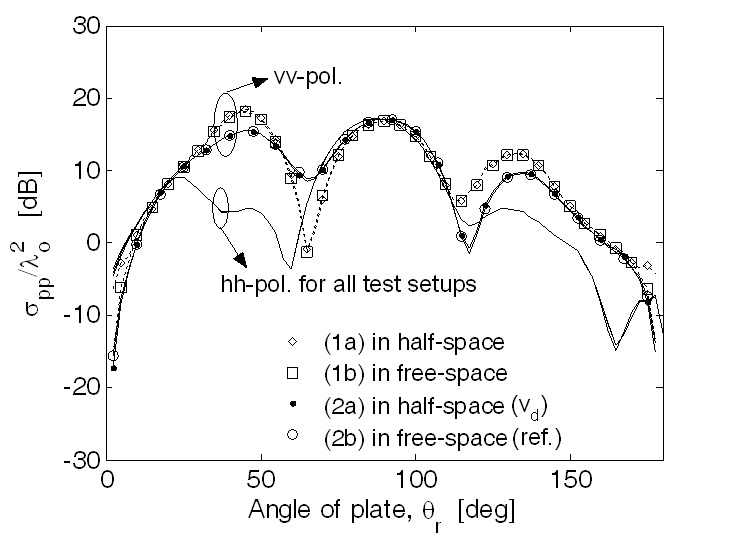
The normalized RCS pattern (line with dots) for the test setup (2a) with virtual vertices agrees well with the reference setup (2b), as shown in Fig. 3. However, the normalized RCS pattern (line with diamonds) for the test setup (1a) without virtual vertices does not agree well with the result (line with circles) of the test-setup (2b) for the vv-polarized backscatter, but it agrees with the test setup (1b) that is distorted by deliberately omitting the boundary edge (line with squares).
In all four test conditions, insertion of the virtual vertices affects the RCS at vertical polarization (vvpol.), while horizontal polarization (hh-pol.) is not affected, so that the four lines are placed on top of each other, as shown in Fig. 3. The current sources vertically passing through the boundary edges are relatively agitated by the ground, so the vv-polarized RCS shows significant errors without the addition of the virtual vertices in this calculation.
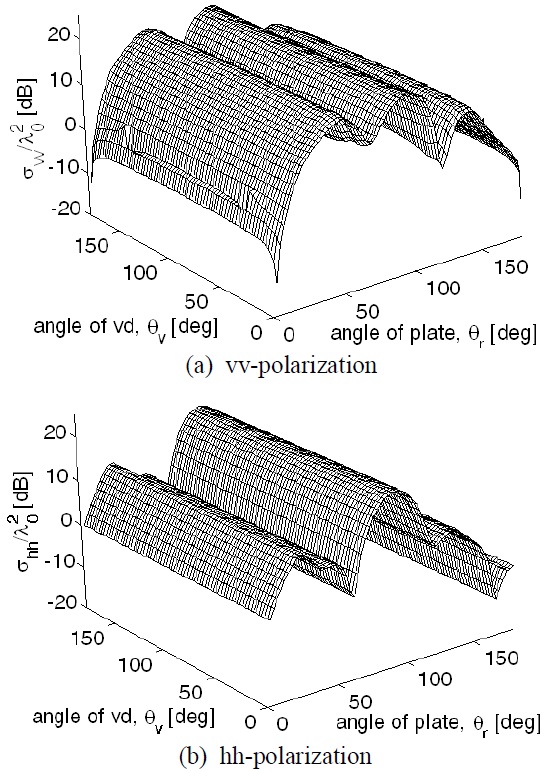
Fig. 4 shows the polarimetric responses of the test setup (2a) with variation of
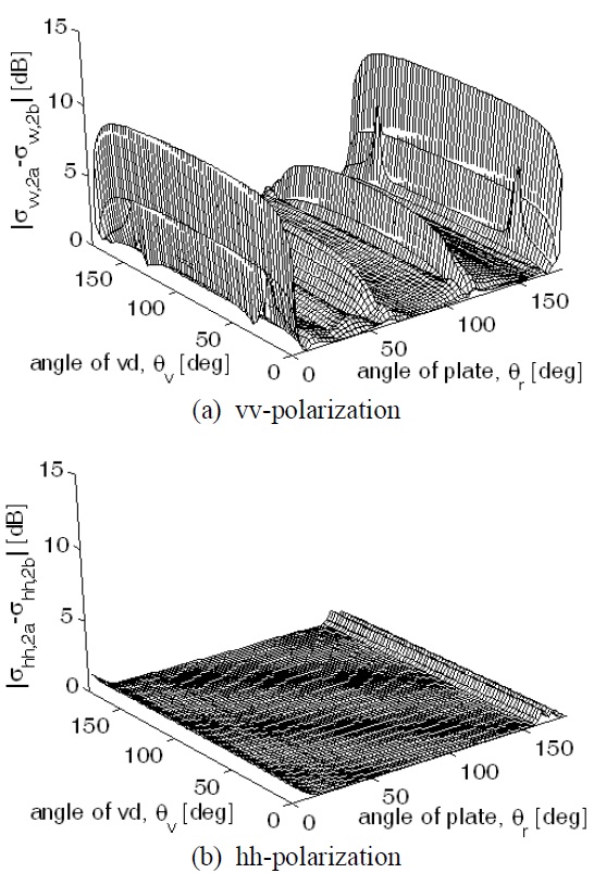
We analyzed the angular effect of the virtual vertices by computing the differences of the RCSs between the two test setups (2a) and (2b) at various angular positions for vv- and hh-polarizations, as shown in Fig. 5. Both test conditions are equivalent, so the test setup (2b) is considered as a reference to examine the computational accuracy of the test setup (2a), which includes the virtual vertices. In the case of vv-polarization, the difference is maximized when
At near
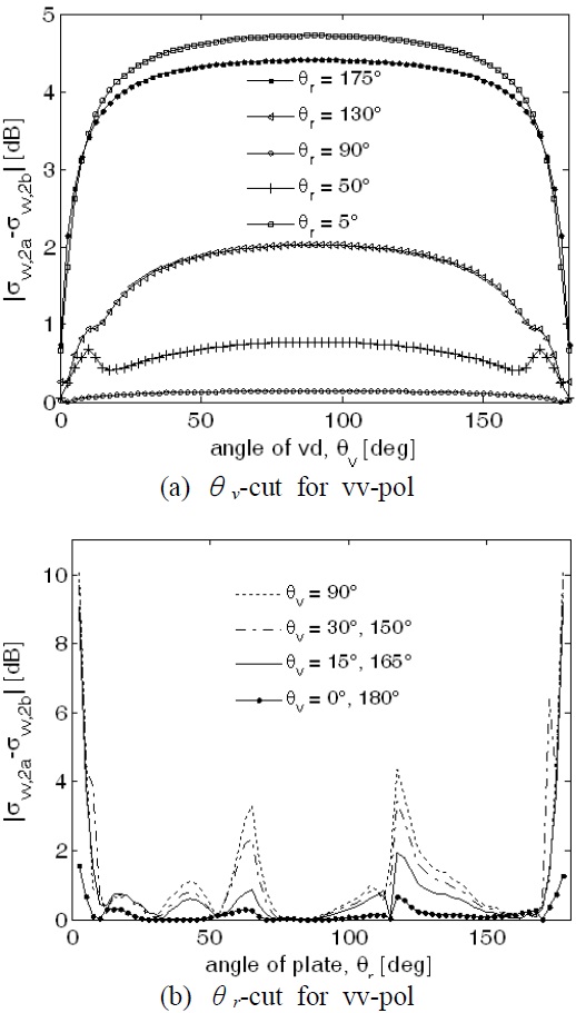
These data were quantitatively analyzed in more detail by drawing the
Fig. 6(a) illustrates the fact that the virtual vertices at
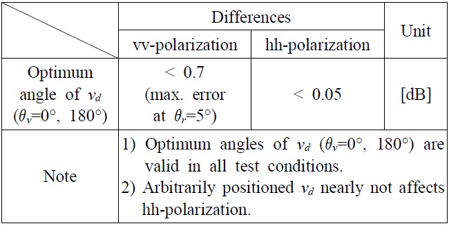
[Table 1.] Angular effect of the virtual vertex.

Angular effect of the virtual vertex.
In addition, this proposed method can be compared with the existing method for the half-space scattering problem. This performance is also summarized as shown in Table 2. In particular, when a metal hemisphere on an infinite ground plane was used as a test target, it consists of two kinds of hemispheres, with and without a bottom side in contact with the interface of the halfspace [4]. Extraction of the singularity caused by the bottom side cells also requires an additional sub-function in the MoM process. This may affect the delay, thereby increasing the processing time and poor accuracy.
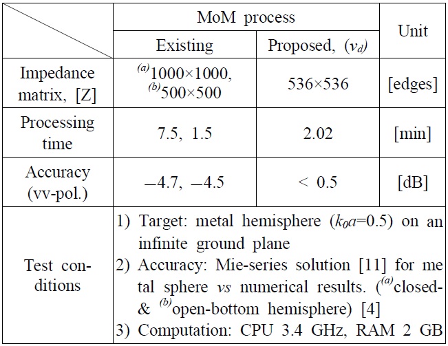
Comparison results of the proposed virtual vertex technique using a metal hemisphere on ground surface.
We investigated the angular effect of the virtual vertices inserted to treat the boundary edges on an infinite conducting surface in this study. A vertical component of the synthesized vector that expresses the current source passing through the problematic boundary edge was identified as contributing to the MoM process for halfspace scattering. Therefore, the angular position of a virtual vertex should be selected to be maximized as a vertical component of the synthesized vector. The optimum angular position of the virtual vertices might lie on the ground plane,
Finally, this proposed technique will contribute to increased accuracy of the numerical model for analyzing the scattering property of scattering particles above the ground surface in the field of microwave remote sensing.