GPS has been used as main navigation system for a variety of aerospace applications. Kalman filter estimation is widely applied to GPS positioning as well as the integration of GPS with inertial navigation system. A conventional Kalman filter is formulated with assumption that both the process and measurement noise are Gaussian white. There are some GPS measurement error modeling studies under SA(Selective Availability) condition[1-4]. Where GPS position measurement error can be modeled as a time correlated low order Gauss-Markov process both continuous and discrete time domain using various parameter identification approaches. Because it is difficult to determine the parameters of Gauss-Markov process in a real-field problem, it is important to estimate of the amount of experimental data recoding time and ensemble average needed for a given required estimation accuracy.
Previous works for kalman filtering methods that consider time-correlated measurement error are categorized in two main approaches. First approach is state augmentation method where the measurement error is augmented into state vector. However, the augmented sate space equation has the perfect measurement with singular measurement covariance matrix that may cause system to become ill-conditioned[5-7]. The second approach uses measurement differencing method to make a new measurement equation corrupted by white noise without time-correlated part[6-9]. Therefore the conventional Kalman filter can be applied to this state and new measurement equation for optimal state estimation. However, In case of multiple measurements, the measurement differencing approach is limited by each measurement should be simultaneously time-correlated.
This paper describes GPS error modeling method for stand-alone single frequency GPS. The relationship between required data recoding time and ensemble average number to satisfy the desired PSD(Power Spectrum Density) estimation error is investigated. It is also shown that the physical parameter of a first or second order dynamic system is related with required data recoding time and ensemble average number. A Kalman filtering method is proposed that consider both correlated/white measurements noise based on characteristics of a stand-alone GPS position and velocity measurements. The performance of the proposed Kalman filtering method is verified via numerical simulation.
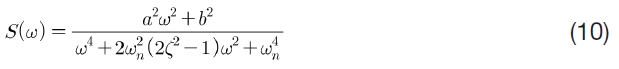
The relationship between PSD and transfer function of single input-output linear time invariant system is described as follows[10].

where

where
is Fourier transform of the
2.2 Normalized PSD Estimation Error
The normalized bias error of PSD estimation can be approximated via Taylor series expansion of expectation of the PDF(Probability Density Function) of a random process
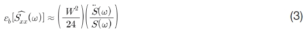
where
The normalized random error of a PSD estimation can be represented using identity that the two degree of freedom chi-square variables have average

where

2.3 Transfer Function Parameter and PSD
An arbitrary transfer function and PSD of the first-order/second-order Gauss Markov process can be represented as follows.
First order:


Second order:

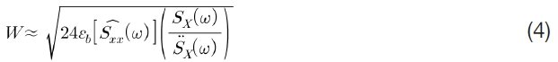
To investigate the relationship between PSD estimation error and resolution bandwidth, we define
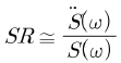
and conservative approach should be applied to determine the frequency for calculation of in Eq. (4).
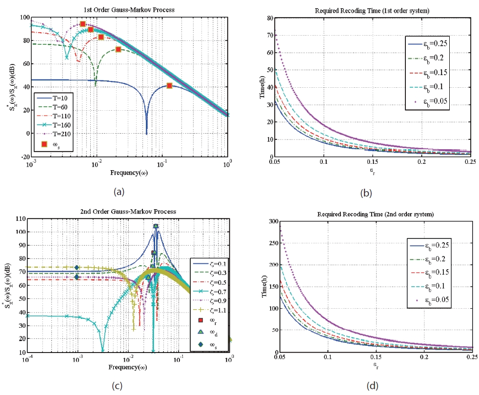
As shown in the Fig. 1. (a)~(b),
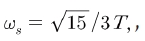
and the second-order Gauss-Markov process has an extreme value of SF depending on the damping ratio. In case of a second-order Gauss-Markov process with lightly damped system(damping ratio range is C<0.3), has a maximum value at the resonance frequency
In case of normally damped system, that has a damping ratio is 0.3 In case of over damped system, that has a damping ratio is C>0.707, SF has a maximum value at the frequency
2.4 Estimation of the PSD and Transfer Function
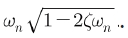
In static condition, the position error dynamic model is identified as a first/second order transfer function, and the velocity error model is identified as a band-limited Gaussian white noise via non-parametric method of a PSD estimation in continuous time domain. Based on quick identification of the position error model of the second order transfer function and its damping ratio
and
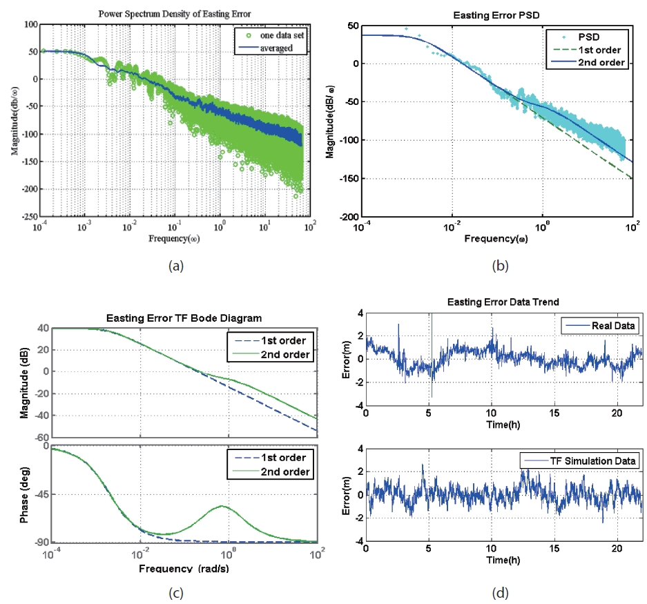
Fig. 2. (a) shows effectiveness of ensemble average of the PSD in frequency domain. In this case, 25 data set of
position error PSD are averaged. Fig. 2. (b) shows fitting of the averaged PSD estimation using nonlinear least square regression method. Fig. 2. (c) bode diagram of the identified transfer function. Fig. 2. (d) shows comparison of the real experimental data and linear simulation of the identified transfer function. In fact, the GPS position error model can be approximated as a first order transfer function within low frequencies with
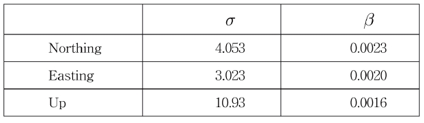
The Identified GPS position error model in NEU coordinate system is summarized in the Table 1.
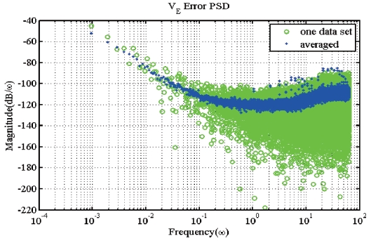
As shown in the Fig. 3, the velocity measurement error PSD has relatively low roll-off ratio and flat magnitude within Nyquist frequency. Therefore it is reasonable to assume that velocity measurement noise is band limited white.
A Kalman filter can be applied to the state-space equation transformed from the error transfer function. The first order transfer function can be obtained as Eq.(11). σ and δ of the first order transfer function corresponding to each axis on NEU coordinate system is summarized in Table 2.

Eq.(11) can be discretized for the sampling time △

3. Kalman Filtering Methodology
The Kalman filtering method is applied for one measurement noise is first order Gauss-Markov process and the other measurement noise is white. Consider the discrete state and measurement equation with both colored measurement noise and white noise.


[Table 1.] Summary of the GPS Position Error Model
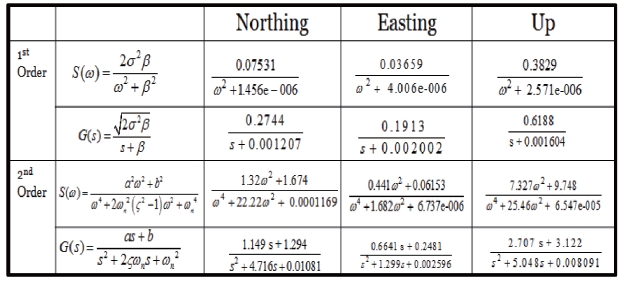
Summary of the GPS Position Error Model
[Table 2.] Summary of the Model Parameters of 1st Order Transfer Function

Summary of the Model Parameters of 1st Order Transfer Function

where
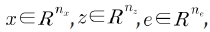
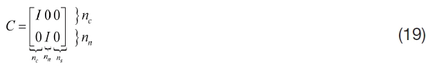
State and measurement equations can be rewritten using Eq.(19) as
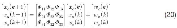
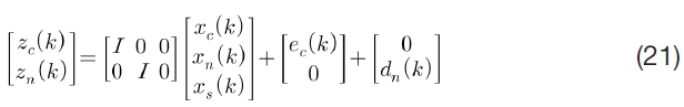
After augmenting time-correlated measurement error state into state vector, state and measurement equations can be rearranged as follows.


where,
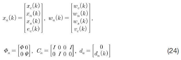
As can be seen in Eq.(24), time-correlated measurement for augmented system model does not contain the white noise. A numerical difference method is used in this paper to avoid the 'perfect measurement condition',which is often the cause of numerical instability. In order to do this, a new measurement vector can be defined as the linear difference of the measurement
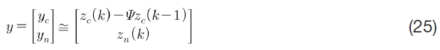
Combination of the augmented state equation and the new measurement equation yields


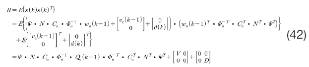
Using Eqs(28)-(29) Eq.(30) is obtained.

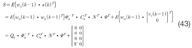
Eq.(27) can be rearranged as,

Eqs.(30)-(31) yields,

Using Eq.(26) and Eq(32), expression on

Time delay of the update on state estimation can be avoided when the measurement can be rewritten using the inverse of the state transition matrix of the augmented state equations:


Now, new parameters

Eq.(22) and Eq.(37) can be simplified as,


where the new measurement noise is white, and
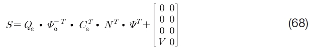
In general, Kalman filter cannot be applied for the case process noise and measurement noise is correlated. Therefore, a generalized Kalman filter is used in this paper in order to obtain optimal estimation that considers both time-correlated measurement noise and white noise. State equation and measurement equation with updates for a generalized Kalman filter are shown in Eq.(44)-(53)[12].


Time Update


Measurement Update


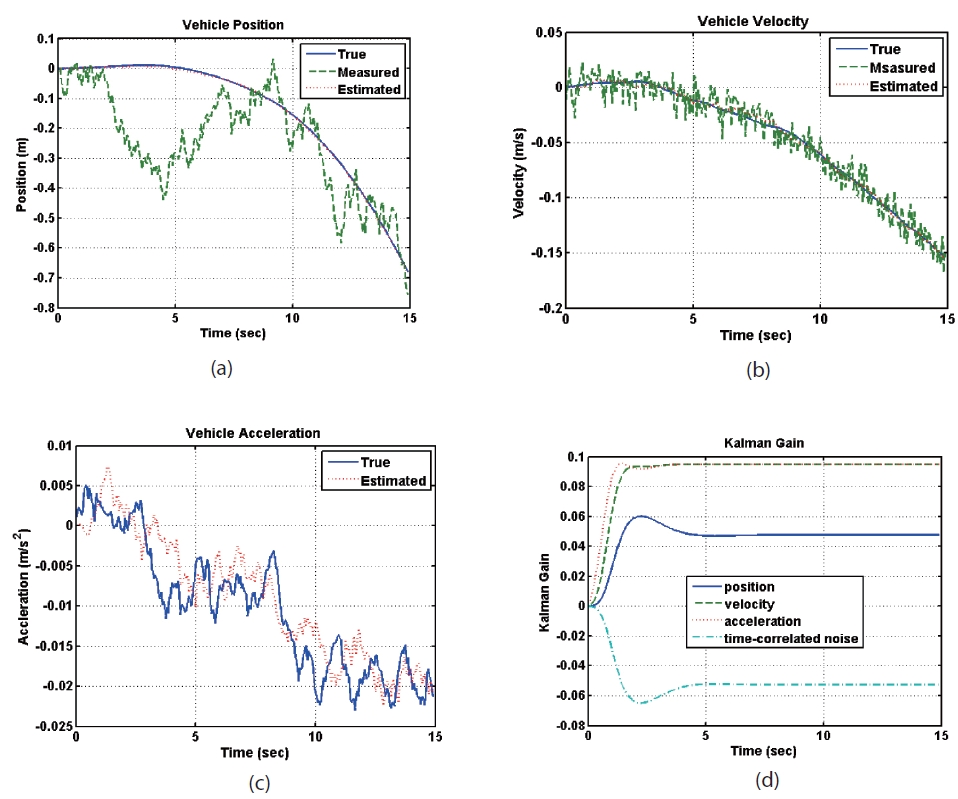
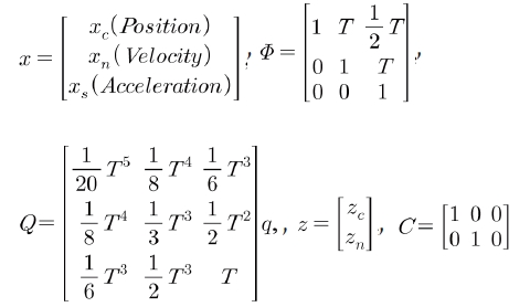
A simple kinematic CWNJM(Continuous White Noise Jerk Model) is considered for numerical simulation. The states are position, velocity and acceleration. It is assumed that the position measurement noise is first-order Gauss- Markov process and velocity measurement noise is white as mentioned in chapter II. Discretized linear dynamic model of CWNJM as follows.


where,
State equation for augmented system can be expressed as,

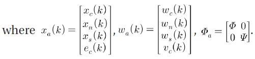
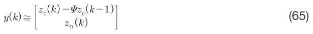
Discretized version of measurement equation can be given by the following equations


Now the state equation and measurement equation are reconstructed so that the generalized Kalman filter can be applied. Parameters for process noise and white noise are set as
Fig. 4. (a) and (b) shows the proposed filter effectively estimates both position corrupted by time-correlated measurement error and velocity corrupted by white noise. Also, the acceleration estimation is appropriate as shown in Fig. 4 (c). In this example, the process noise covariance is set relatively small value to show the estimate with respect to noise magnitude during small time window. It should be noted that the initial states are assumed to be known. Actually, this proposed Kalman filter de-correlates the time correlated measurement error of the position using velocity information which is not corrupted by time correlated noise, but by white noise. Moreover, using the velocity information and simple kinematics, we can get acceleration estimation without additional measurements.
In this paper, a dynamic modeling method for the velocity and position information of a single frequency stand-alone GPS receiver is described. The relationship between ensemble averages, required data recoding time and PSD estimation error that satisfy the given error bound is described. Also, analysis on transfer function parameters of a first and a second order linear system with respect to PSD error is described. A Kalman filter is proposed that consider both correlated/white measurements noise based on identified GPS error model. The proposed Kalman filter is derived from the fusion of the state augmentation approach and measurement differencing approach. The performance of the proposed Kalman filter is verified via numerical simulation. Using this filter, the time correlated position error of the GPS measurement is effectively decorrelated via its own GPS velocity information without any additional sensors. In near future, the proposed Kalman filtering method will be formulated for more general cases and applied to the precise navigation of moving vehicles.