Composite materials have various applications in many engineering structural fields. Especially, aerospace structures require high stiffness and strength to weight ratio. These applications have required accurate prediction of the thermo-mechanical behavior of composite laminates for the design and analysis of structural composite. Therefore, advanced composites have been used continuously and have been expanded in their application for the last three decades. Numerous theories (Pagano, 1969; Pagano, 1970; Reddy, 2004) have been developed for the accurate analysis of laminated composite structures. Several equivalent single layer (ESL) plate theories (Reddy, 2004) are developed by assuming the form of the in-plane displacement field as a linear combination of unknown functions and the thickness coordinate. The first ESL theory is a classical laminated plate theory (CLPT), based on the Kirchoff-Love plate assumption that the in-plane displacement remains normal to the centerline of the plate after deformation. Improved theory over CLPT is a first-order shear deformation theory, which considers the transverse shear deformation of the plate which requires the shear correction factor. Even though the FSDT is more reliable than the CLPT, it still cannot accurately predict the mechanical behaviors for the laminated composite plates. Thus, more advanced theories have been required, and a series of the smeared higher order theories (Lo et al, 1977; Reddy, 1984) have been developed for the laminated composite plates. For instance, the third-order shear deformation theory uses a cubic polynomial for the in-plane displacement field. In TSDT, there is no need to use the shear correction factor. Among the advanced theories, efficient higher order plate theory (EHOPT), developed by Cho and Parmerter (1993), demonstrates the best performance among displacement-based zig-zag theories. It has been recognized that the zig-zag pattern of in-plane displacement provides the accuracy analysis of deformation and stress.
Meanwhile, in all of the above ESL theories, the material properties of composite laminates have been considered as linear elastic materials. In reality, composite laminates are inhomogeneous materials which are composed of a viscoelastic matrix and elastic fibers as reinforcement (Yi, Pollock, Ahmad and Hilton, 1994). Hence, like other viscoelastic materials, the mechanical behavior of fiber reinforced composites leads to creep strain, stress relaxation and time-dependent failure. These viscoelastic behaviors are critical when the composite laminates are in high temperature or vibrating conditions. Several researches (Hilton and Yi, 1993; Aboudi and Cederbaum, 1989) have analyzed the dynamic response of composite laminates considering the viscoelastic effects. For example, Srinatha and Lewis (Srinatha and Lewis, 1981) suggested a numerical procedure which solved an integral problem using the trapezoidal integration method for the Boltzmann superposition integral. As a result, the accuracy of the results depends on a time step Δt. However, it requires extensive computational time to obtain the reliable results by reducing the size of each time step, especially for long-term problems. Other researchers (Chen, 1995; Hilton and Yi, 1993) solved the problem of computational cost by using the Laplace transformation for a viscoelastic beam. The results in the real time domain were obtained by the inverse Laplace transformations based on numerical calculation.
In the present study, the mechanical behavior of viscoelastic composite laminates is investigated using the Laplace transformation based on the FSDT and TSDT. By applying Laplace transformation instead of the direct time integrations of the Boltzmann superposition integral and directly inversing the equations in the Laplace domain to the real time domain, the accuracy increases significantly as much as that of elastic counterparts. In addition, since the viscoelastic constitutive equation has the form of integration, the top and bottom stress free conditions cannot be directly applied in the TSDT model. Thus, based on the Laplace transformation, top and bottom stress free conditions are successfully applied in the Laplace domain, which makes the theoretical formulation very simple. The present theory considers viscoelasticity in two basic models: Maxwell and Kelvin for viscoelastic phenomena such as creep, cyclic creep and recovery. More complex models with extended Prony series can be developed from these basic models.
The presented and discussed numerical results focus on: (1) the comparison of deflections by using the FSDT and TSDT for elastic composite laminates; (2) the deflection of both elastic and viscoelastic composite laminate; (3) the influence of viscoelastic coefficients to dynamic responses of composite laminates; (4) the in-plane displacement of viscoelastic composite laminates.
2.1. Constitutive equation for linear viscoelastic material
Instead of Hook’s law, the stress-strain relation for linear viscoelastic materials can be expressed by Boltzmann superposition integral equations:
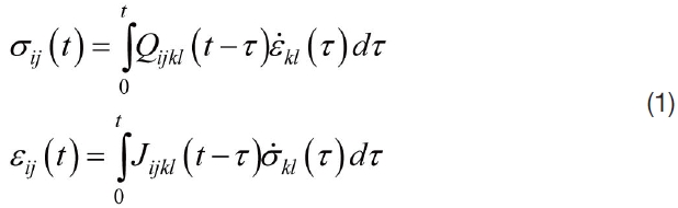
where

where the relaxation modulus
In the present study, the viscoelastic material is modeled by following both Maxwell and Kelvin models. The relaxation modulus for the Maxwell model (Eq. 3) and the compliance modulus for the Kelvin model (Eq. 4) are expressed as time-
dependent simpler forms:


By taking the Laplace transform with respect to time, the Boltzmann superposition integral equation in the Laplace domain can be derived as:

where ( )* are the parameters in the Laplace domain.
It is well recognized that the form of the Boltzmann superposition integral equation in the Laplace domain for viscoelastic material is similar to that of Hook’s law in linear elastic constitutive equations. Hence, it is possible to solve the problem of viscoelastic laminate in the Laplace domain with the same elastic counterpart.
2.2. First-order shear deformation theory
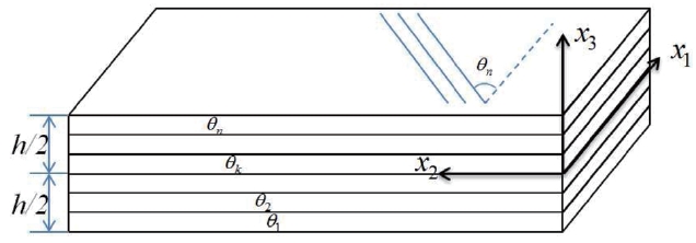
In this paper, we consider a linear plate model with the thickness
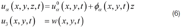
where
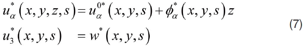
Due to the linearity of the Laplace transform, the displacement field in the Laplace domain can be written as,
In the present theory, the virtual work principle for quasistatic viscoelastic problems is described as:
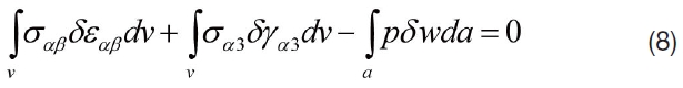
where
Substituting the displacement fields into the virtual work principle and applying Laplace transform, the equilibrium equations can be obtained:
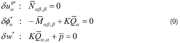
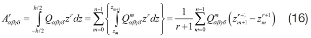
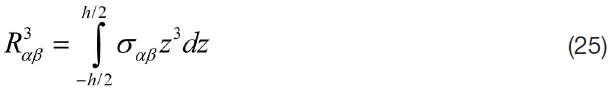
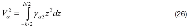
where stress resultants are defined as follows:
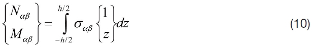
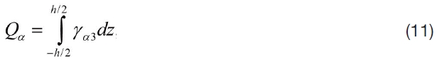

The resultants in the Laplace domain can be expressed as follows:


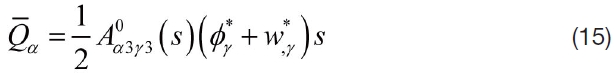
where stress resultants
For both static and harmonic loadings, the cylindrical bending behavior of the composite plate is analyzed. Thus, all of the equilibrium equations are reduced to the one dimensional form. The displacement variables are assumed as a trigonometric form by considering the simply supported boundary. In the time domain, the displacement and transverse load can be chosen to be of the forms:
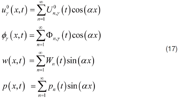
where
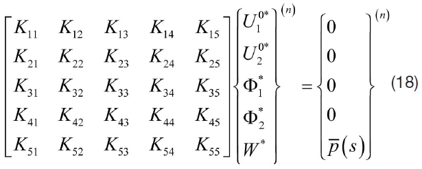
where [
By applying the inverse Laplace transform to Eq. (18), the algebraic relations in the real time domain can be obtained as follows:
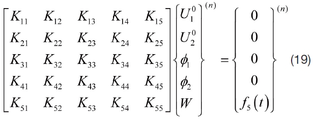
where
From Eq. (19), the solutions of (
2.3. Third-order shear deformation theory
Following the third-order transverse deformation, the time dependent displacement can be expressed in the following forms:
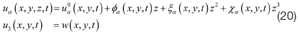
where
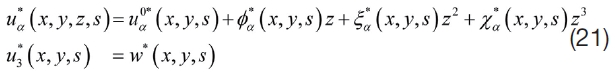
Being identical to Eq. (6)-(7), the displacement fields in the Laplace domain can be written as:
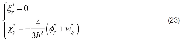
The number of the unknown variables is reduced by applying top and bottom surface traction free boundary conditions as follows:

Similar to FSDT analysis, substituting the displacement fields into the virtual work principle and applying Laplace transformation, the equilibrium equations can be obtained as follows:
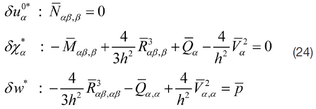
where the added stress resultants are defined as:

The resultants in the Laplace domain can be expressed as follows:
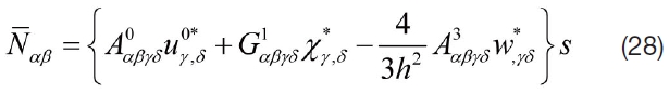
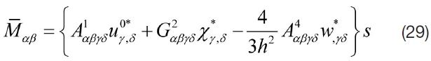
where stress resultants
Executing the same procedure as the FSDT case, the algebraic relations can be obtained as follows:
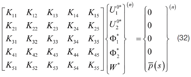
where [
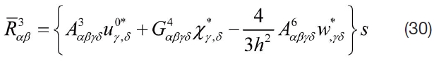
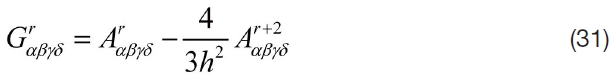
By applying the inverse Laplace transform to Eq. (32), the algebraic relations can be obtained as follows:
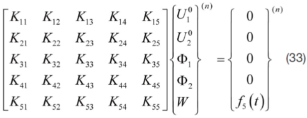
From Eq. (33), the solutions of (
3. Numerical results and discussion
To compare the present analysis with the results of the previous study and other theories, the [0/90/0] laminated composite plate is chosen as an illustrative numerical example. The material properties of the ply are:
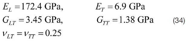
where

To show the influence of the viscoelastic coefficient to mechanical behavior especially transient time, the coefficients

for both static and harmonic loadings.
The displacements are normalized by the following nondimensional values:
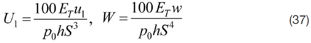
where
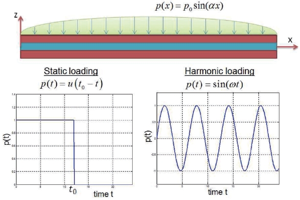
The numerical examples consider both static and harmonic loads which are shown in Fig. 2. The static loading, which is constant with respect to time, is presented as follows:

where

where
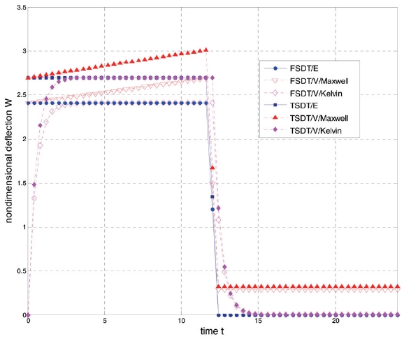
3.1. Numerical result for static loading
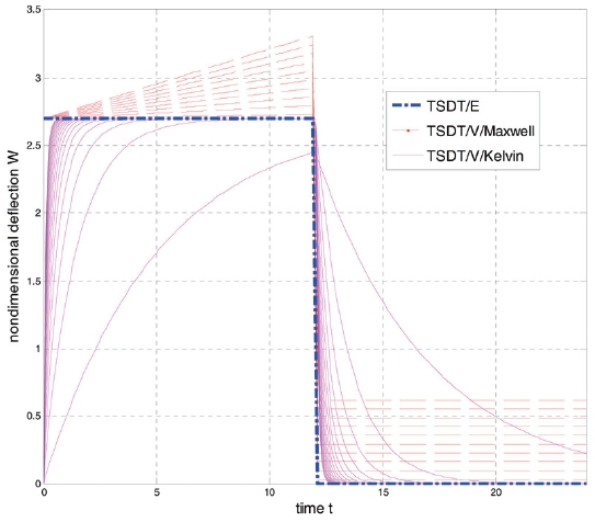
Fig. 3 shows the nondimensional deflection
Kelvin model, at transient time, the value of deflection
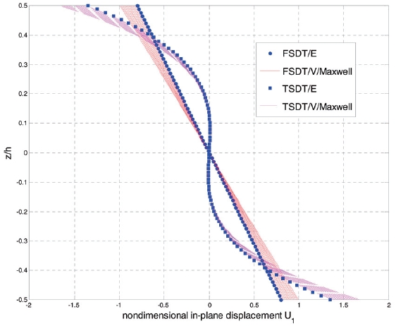
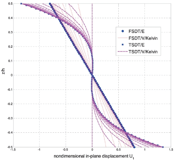
Fig. 4 shows the time-dependent nondimensional inplane displacement
displacement
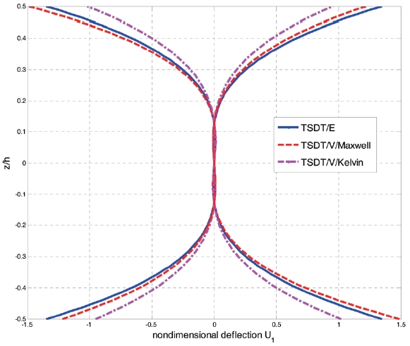
Fig. 6 shows the influence of viscoelastic coefficients for the Maxwell and Kelvin model to the deflection of the midplane for the TSDT. For the Maxwell model, the angle
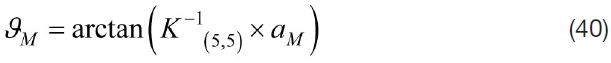
where
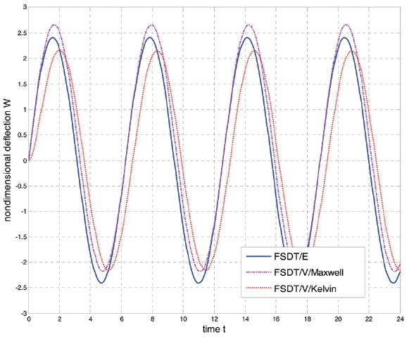
3.2. Numerical result for harmonic loading
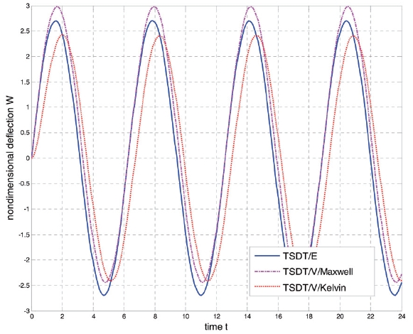
Fig. 7 and 8 show the time-dependent nondimensional deflection
is represented as a continuous line, the displacement has the same phase with the harmonic loading Δ
Fig. 9 presents the time-dependent nondimensional in-plane displacement
viscoelastic response for both Maxwell and Kelvin models are distinguished clearly. The fluctuation region of the elastic case is limited by two continuous lines; the one of viscoelastic case with the Maxwell model is limited by the discontinuous line, and the one with the Kelvin model is limited by the two dot-dashed lines. The amplitude of
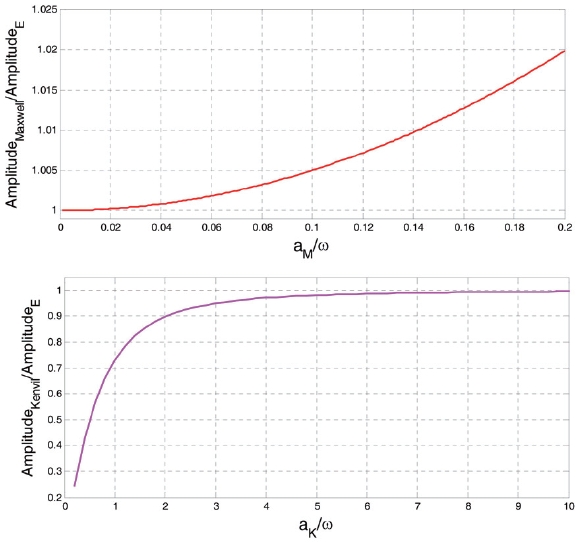
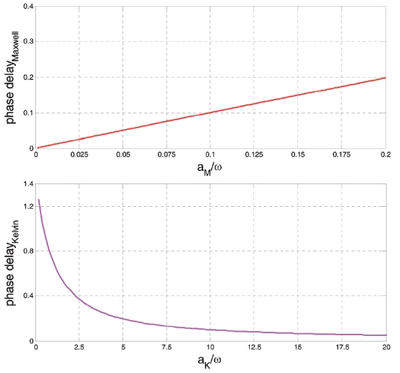
Fig. 10 shows the effect of the viscoelastic coefficient to the amplitude of deflection in the case of harmonic loading. The upper figure is for the Maxwell model and the lower one is for the Kelvin model. With the small value of
The mechanical behaviors of linear viscoelastic composite laminates have been analyzed by applying the Laplace transform without any integral transformation or any time step scheme. The numerical examples for static and harmonic loading under the quasi-static assumption show the creep responses of viscoelasticity for both the FSDT and TSDT cases. For the harmonic loading, the results of both basic models demonstrate the phase delay and the change of amplitude of deflection compared to the elastic one. For static loading, the Kelvin model has a better analysis for creep responses than that of the Maxwell model, especially in transient time.
For more efficient analysis, a higher-order cubic zig-zag theory such as efficient higher order plate theory (Cho, 1993), needs to be developed in the environment of viscoelastic behavior. In addition, a time-dependent relaxation modulus needs to be expresses through general Prony series which was developed in the present study for basic Maxwell and Kelvin models. These are currently under process.
>
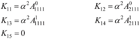
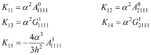
Appendix A. Components of the stiffness matrix K of FSDT:
♣ The first row of stiffness matrix
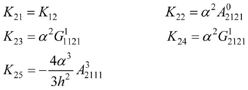
♣ The second row of stiffness matrix
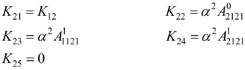
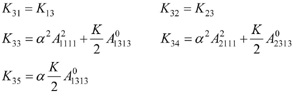
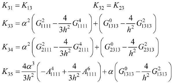
♣ The third row of stiffness matrix
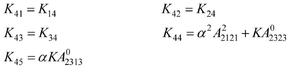
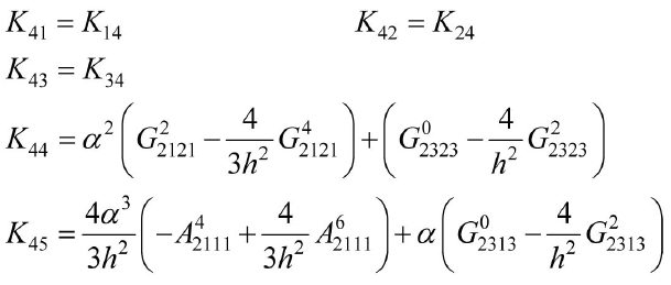
♣ The fourth row of stiffness matrix
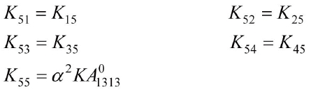
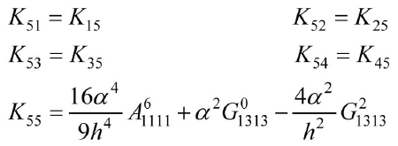
♣ The fifth row of stiffness matrix
>
Appendix B. Components of the stiffness matrix K of TSDT:
♣ The first row of stiffness matrix K:
♣ The second row of stiffness matrix K:
♣ The third row of stiffness matrix K:
♣ The fourth row of stiffness matrix K:
♣ The fifth row of stiffness matrix K:
>
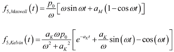
Appendix C. The functions of f5(t):
♣ For static loading
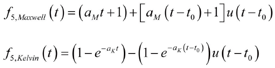
♣ For harmonic loading