Missiles suffer from flight instability problems at high angles of attack, since the vortex flow over a fuselage causes lateral force to the body [1]. To overcome this problem at high angles of attack, the development of a real time vortex controller is needed. For developing real time controllers, reduced order modeling techniques are surely necessary, since full simulation of the system is extremely time consuming. Aerodynamic forces can be determined by simple matrix algebra using the ROM technique. The POD method is one of the most well-known techniques for modeling low order models that represents the original full-order model [2]. The basic idea of this method is to project N-dimensional state spaces onto an M-dimensional subspace, where M is much bigger than N. After the POD procedure, a system identification technique is performed to estimate POD modal amplitudes. An artificial Neural Network-Auto Regressive Exogenous (ANN-ARX) method, which estimates POD modal amplitude more accurately and faster than using Galerkin projection or stochastic estimation [3], is used in this paper. The reduced order model (ROM) is completed by organizing the POD method and an ANN-ARX model. After building a ROM, direct adaptive control law is chosen to close the loop. This method of control will help to reduce the vortex shedding and to achieve a desired closed loop flow state [4].
2.1 Proper Orthogonal Decomposition (POD)
POD is used to determine an optimal basis for representing a given data set. The goal of this method is to obtain an orthogonal basis, so that almost every member of the data can be decomposed relative to the basis. Therefore, the original higher order system can be represented by the combination of the minimum number of aerodynamic modes. That is, using the method, flow data, , which are functions of space and time, can be represented as follows [2] :
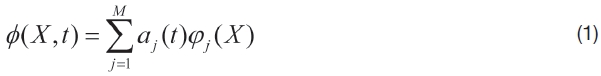
where

To obtain POD basis, φ, a snapshot method, is widely used for its convenience [5]. In this approach, full CFD simulation is performed initially. During this process, snapshots which have fluid information are recorded at selected times. Finally, a singular value decomposition of the snapshot matrix is performed to get POD modes.
2.2 Artificial Neural Network-Auto Regressive Exogenous (ANN-ARX)
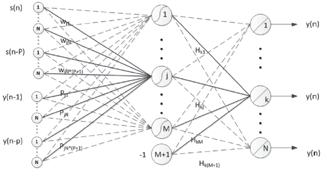
ANN-ARX is a system identification method which combines an artificial neural network and an auto-regressive exogenous model. It estimates POD modal amplitude more accurately and faster than using Galerkin projection or stochastic estimation [3]. The method can maximize the effectiveness of the real time feedback flow controller, since
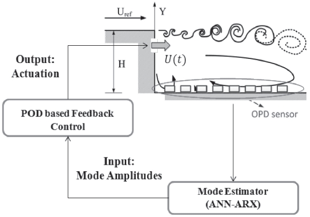
it excludes the CFD analysis for Navier-Stokes equation. The model was developed using a multi-layer perceptron, which contains more than 1 hidden layer, to increase the ability to estimate nonlinear behavior [6]. An ANN-ARX model was combined with the POD method for reduced order modeling of vortex flow. Schematics of the ANN-ARX model, which estimates POD modal amplitude, is shown in Fig. 1.
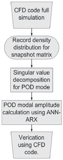
The density gradient, which was calculated by CFD analysis, was applied to the POD method to calculate POD mode and POD modal amplitude. ROM was completed by organizing the POD method and ANN-ARX model, which generates POD modal amplitudes. The flow chart is shown in Fig. 2.
2.3 Direct model reference adaptive control
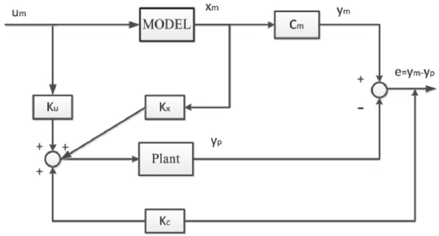
Model reference control is based upon matching the response of a system to that of a reference model. The control system can be designed so that the inputs to the plant drive the outputs of the plant to follow the outputs of the model. A block diagram of the model reference control system is shown in Fig. 3.
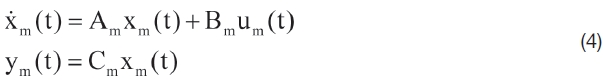
The system for the continuous linear model reference control has the form [7]:
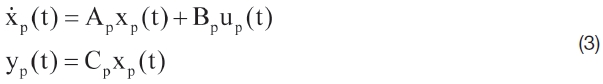
where
where
When perfect output tracking occurs, the ideal plant which satisfies the same dynamics as the real plant can be written as linear functions of the model state and model input, which has the form:
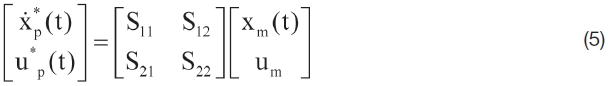
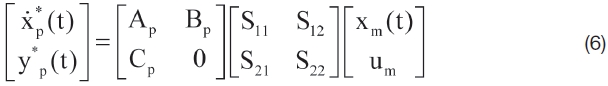
where

where
3. Backward facing step wall model
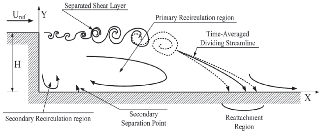
The backward facing step wall model, which is the target model of this research, is shown in Fig. 4. A Spalart- Allmaras turbulent model based on the DDES method was used to simulate the unsteady turbulent flow over a 3-D backward facing step [8]. The physical properties of the backward facing step wall model were the same as that of Driver and Seegmiller’s experiment [9]. The height of the step is marked as and the heights of inlet and exit are 8H and 9H, respectively. The isothermal viscous wall boundary condition is applied to the top and bottom wall, and the periodic boundary condition is applied in the z-direction. The inlet and outlet boundary were set as the specified turbulent boundary layer and the constant pressure outflow boundary condition, respectively. The properties of the model are represented in table 1.
[Table 1.] The properties of the backward facing step wall flow model
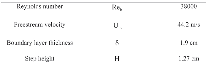
The properties of the backward facing step wall flow model
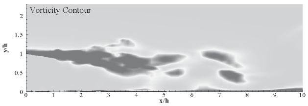
As shown in Fig. 5, the instantaneous vorticity contour displays small vortice structures breaking up from the shear layer. In order to build a flow database, a number of numerical simulations are performed with actuating amplitude and frequency for open-loop sinusoidal suctionblowing. Blowing and suction actuator was implemented at the edge of the step for open-loop control. The length of the actuator inlet is 0.08H and the actuator was installed parallel with the ground. The velocity, Ua of the actuator was set as

where, A0 is the amplitude and ω is the frequency of the actuator. The actuation frequencies of the open loop cases are determined as 200Hz, 300Hz, and 400Hz. The actuation amplitudes are determined as 1%, 2% and 3% of the freestream velocity.
3.2 ROM of the backward facing step wall
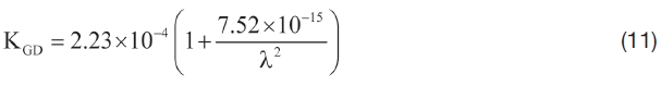
To represent the extent of flow wake, the Optical Path Difference (OPD) was used in this research. Based on the Gladstone Dale relation, the Optical Path Length (OPL) was calculated to obtain the OPD [10]. Assuming that the optical beam is propagated in the y-direction, an average OPL in the x-z plane is subtracted, and the OPD can be written as

where,

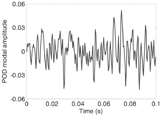
OPD is linearly dependent on the fluid density. Time history of OPD was arranged in a snapshot matrix and it was applied to the POD method to calculate POD mode and modal amplitude, as described in section 2.1. POD modes for all open loop cases were calculated, and the 1st POD modal amplitude for the baseline case is shown in the Fig. 6.
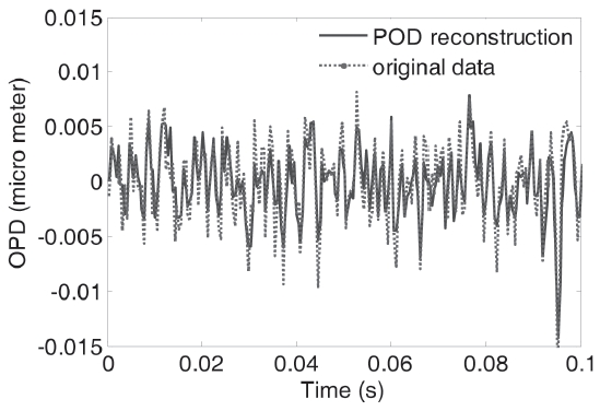
Fig. 7 shows the comparison between the original CFD result and the reconstruction data using 2 POD modes. Openloop control case; and , was chosen for the comparison with CFD result and POD reconstruction. The results show good agreement between the two modes. From the results, it is verified that two POD modes are suitable for reduced order modeling.
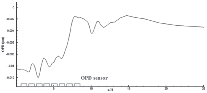
ROM was completed by applying an ANN-ARX method to estimate POD modal amplitudes. At first, POD modal amplitude was calculated by the POD method and CFD results. Second, error back-propagation was applied for ANN-ARX modeling by appointing the actuator velocity as input, and the OPD data from sensors as output. Fig. 8 shows the OPD distribution among at an arbitrary time, and OPD sensors were placed at . After ANN-ARX estimates the OPD data from sensors, a mode estimator was constructed to estimate POD modal amplitude.
The process which identifies the system using error backpropagation is called training, and the number of training cases is one of the most important parameters of the ROM. Training cases used in this study are shown in the table 2. There are 10 cases depending on the amplitude and the frequency of the actuator, as represented in equation (3) including the baseline case. Nine cases were trained and one case was used as a validation case.
[Table 2.] Summary of cases. O: training cases, X: validation case
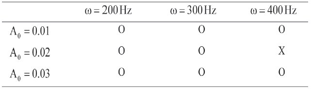
Summary of cases. O: training cases, X: validation case
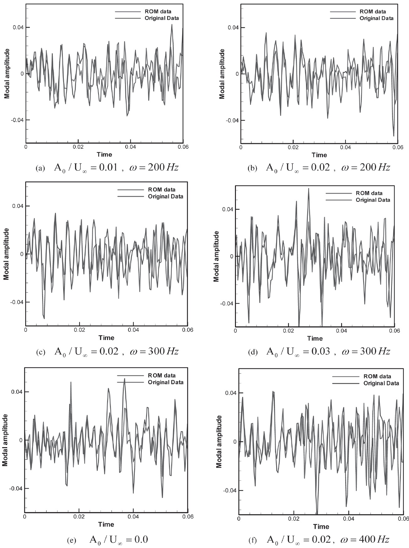
Fig. 9 shows the comparison of the results from the use of ANN-ARX and CFD analysis. Design cases and off-design cases were compared in Fig. 9. Fig. 9 (a) ? (d) shows the open loop cases trained by specified amplitude and frequency, as represented in table 2. Fig. 9 (e) shows the baseline case and fig. 9 (f) shows the off-design case for validation. The figures show relatively good agreement between ANN-ARX and CFD analysis for the design cases, however, the error became larger for the off-design cases. From the results, the ROM model predicted the tendency of the CFD analysis, which is the most important precondition for real time feedback flow control using ROM models.
ROM constructed by the POD and ANN-ARX methods was used for real time vortex control of the backward facing step wall model. A direct model reference adaptive controller was chosen for the feedback controller, and it was
designed to control the 1st POD modal amplitude, since it contains the greatest energy of the system. A block diagram of the controller and the schematics of the control model are shown in Fig. 10.
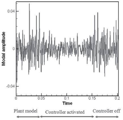
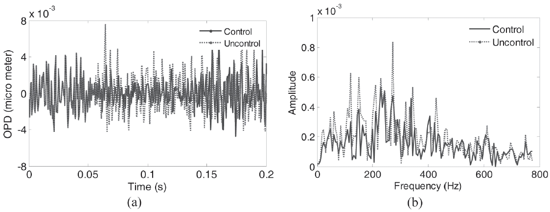
The control algorithm was applied to the ROM. Two POD modes were used for reconstruction of the wake flow. POD modal amplitudes were calculated when the baseline flow blows during 0 ~ 0.05 s and the controller actuated at 0.05 s. Finally, the controller was turned off and unforced flow redeveloped at 0.15 s. The control results for POD modal amplitude are shown in Fig. 11. It shows that the direct model reference adaptive controller activated effectively when it was turned on. The OPD of the control results was reconstructed using two POD modal amplitudes and their spatial modes, as mentioned at section 3.2. The OPD at the point of interest, is plotted in Fig. 12 (a) and a spectral analysis of the OPD is plotted for the feedback flow control and uncontrolled case in Fig. 12 (b). The OPD variation shows that the OPD was reduced during the feedback control, and the dominant frequency of the feedback flow control signal corresponds to an uncontrolled signal.
In this research, a Spalart-Allmaras turbulent model based DDES method was used to simulate the unsteady turbulent flow over a 3-D backward facing step. Since full simulation of the system is extremely time consuming, ROM were constructed by POD and ANN-ARX methods to develop a real time controller. Direct model reference adaptive control law was chosen to close the loop to reduce the vortex shedding, and to achieve a desired closed loop flow state. Designed feedback controller was used effectively to reduce the OPD of the BFS model, since the controller reduced the 1st POD modal amplitude of the wake flow.