Code division multiple access (CDMA) has been widely used and accepted for wireless access in terrestrial and satellite applications. CDMA cellular systems use state of the art digital communication techniques and build on some of the most sophisticated aspects of the modern statistical communication theory. The CDMA technique has significant advantages over the analog and conventional time division multiple access (TDMA) system. CDMA is a multiple access (MA) technique that uses spread spectrum modulation where each user has its own unique chip sequence. This technique enables multiple users to access a common channel simultaneously.
Multiuser direct sequence (DC)-CDMA has received wide attention in the field of wireless communications [1,2]. In CDMA communication systems, several users are active on the same fringe of the spectrum at the same time. Therefore, the received signal results from the sum of all the contributions from the active users [3]. Conventional spread spectrum mechanisms applied in DS-CDMA are severely limited in performance by multiple access interference (MAI) [1,4], leading to both system capacity limitations and strict power control requirements. The traditional way to deal with such a situation would be to process the received signal through parallel devices.
Verdu [5] proposed and analyzed the optimum multiuser detector and the maximum likelihood (ML) sequence detector, which, unfortunately, is too complex for practical implementation, since its complexity grows exponentially as the function of the number of users. Although the performance of the multiuser detector is optimum, it is not a very practical system since the number of required computations increases by 2k, where k is the number of users to be detected. Multiuser detectors suffer from their relatively higher computational complexity that prevents CDMA systems from adapting this technology for signal detection. However, if we could lower the complexity of the multiuser detectors, most of the CDMA systems would likely take advantage of this technique in terms of its increased computing power and superior data rate.
In this paper, we employ a new scheme that observes the coordinates of the constellation diagram to determine the location of the transformation points. Since most of the decisions are correct, we can reduce the number of the required computations by only using the transformation matrices on those coordinates which are most likely to lead to an incorrect decision. By doing this, we can greatly reduce the unnecessary processing involved in making decisions concerning the correct regions or the coordinates. Our mathematical results show that the proposed approach successfully reduces the computational complexity of the optimal ML receiver.
The rest of this paper is organized as follows. Section II describes the state of the art research that has already been done in this area. Section III presents both the original ML algorithm and the proposed power efficient (PE) algorithm along with a comprehensive discussion of their computational complexities. The numerical and simulation results are presented in Section IV. Finally, we conclude the paper in Section V.
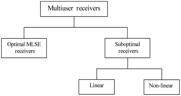
Multiuser receivers can be categorized in the following two forms: optimal maximum likelihood sequence estimation (MLSE) receivers and suboptimal linear and nonlinear receivers. Suboptimal multiuser detection algorithms can be further classified into linear and interference cancellation type algorithms. The figurative representation of the research work that has been done so far in this area is presented in Fig. 1. The optimal multiuser wireless receiver consists of a matched filter followed by an ML sequence detector implemented via a dynamic programming algorithm. In order to mitigate the problem of MAI, Verdu [6] proposed and analyzed the optimum multiuser detector for asynchronous Gaussian MA channels. The optimum detector searches for all the possible demodulated bits in order to locate the decision region that maximizes the correlation metric given by [5]. The practical application of this mechanism is limited by the complexity of the receiver [7]. This optimum detector outperforms the conventional detector, but unfortunately its complexity grows exponentially in the order of
Much research has been done to reduce the computational complexity of this receiver. Agrell and Ottosson [8] proposed a new ML receiver that uses the neighbor descent (ND) algorithm. They implemented an iterative approach using the ND algorithm to locate the region where the actual observations belong. In order to reduce the computational complexity of optimum receivers, the iterative approach uses the ND algorithm that performs MAI cancellation linearly. The linearity of their iterative approach increases noise components at the receiving end. Due to the enhancement in the noise components, the signal to noise ratio (SNR) and bit error rate (BER) of the ND algorithm are more affected by the MAI.
Several tree-search detection receivers have been proposed in the literature [9,10], to reduce the computational complexity of the original ML detection scheme proposed by Verdu. Specifically, [9] investigated a treesearch detection algorithm, where a recursive, additive metric was developed in order to reduce the search complexity. Reduced tree-search algorithms, such as the wellknown M- and T-algorithms [11], were used by [10] to reduce the complexity incurred by the optimum multiuser detectors.
To make an optimal wireless receiver that provides minimum mean square error (MMSE) performance, we need to provide some knowledge of interference such as phase, frequency, delays, and amplitude for all users. In addition, an optimal MMSE receiver requires the inversion of a large matrix. This computation takes a relatively long time and makes the detection process slow and expensive [2,7]. On the other hand, an adaptive MMSE receiver greatly reduces the entire computation process and gives an acceptable performance. Xie et al. [12] proposed an approximate MLSE solution known as the presurvivor processing (PSP) type algorithm, which combined a tree search algorithm for data detection with the aid of the recursive least square (RLS) adaptive algorithm used for channel amplitude and phase estimation. The PSP algorithm was first proposed by Seshadri [13] for a blind estimation in single user inter-symbol interference (ISI)-contaminated channels.
III. PROPOSED LOW-COMPLEXITY PE ALGORITHM
We consider a synchronous DS-CDMA system as a linear time invariant (LTI) channel. In an LTI channel, the probability of variations in the interference parameters, such as the timing of all users, amplitude variation, phase shift, and frequency shift, is extremely low. This property makes it possible to reduce the overall computational complexity at the receiving end. Our PE algorithm utilizes the complex properties of the existing inverse matrix algorithms to construct the transformation matrices and to determine the location of the transformation points that may occur in any coordinate of the constellation diagram. The individual transformation points can be used to determine the average computational complexity.
The system may consist of
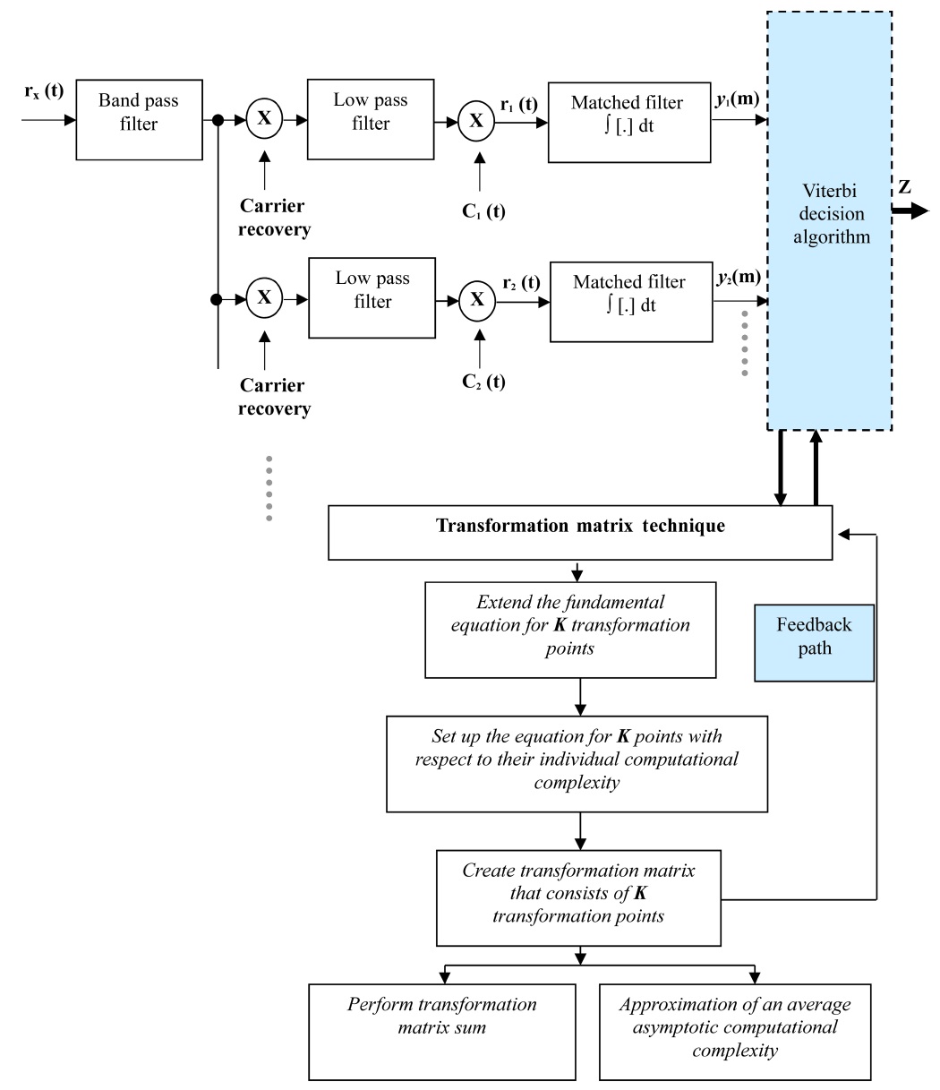
The cross correlation can be reduced by neglecting the variable delay spreads, since these delays are relatively small as compared to the symbol transmission time. To detect signals from any user, the demodulated output of the low pass filter is multiplied by a unique signature waveform assigned by a pseudo-random number generator. It should be noted that we extract the signal using the match filter followed by a Viterbi algorithm.
>
A. Original Optimum Multiuser (ML) Receiver
The optimum multiuser receiver exists and permits to relax the constraints of choosing the spreading sequences with good correlation properties at a cost of increased receiver complexity. Fig. 2 shows the block diagram of an optimum receiver that uses a bank of matched filters and an ML Viterbi decision algorithm for signal detection. It should be noted in Fig. 2 that the proposed PE algorithm is implemented in conjunction with the Viterbi decision algorithm with the feedback mechanism. To detect a signal from any user, the demodulated output of the low pass filter is multiplied by a unique signature waveform assigned by a pseudo-random number generator.
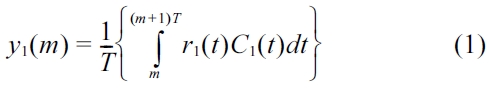
When the receiver wants to detect the signal from user- 1, it first demodulates the received signal to obtain the base-band signal. The base-band signal multiplies with user-1’s unique signature waveform,
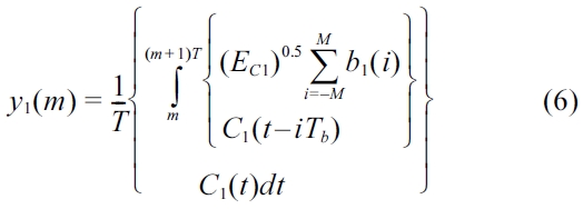
The received signals
where
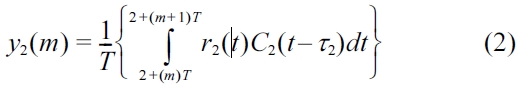
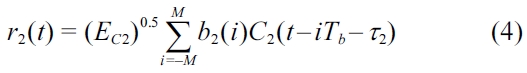
The received signals
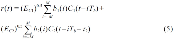
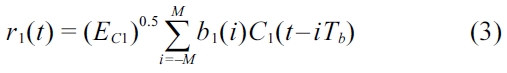
Substitute (5) as an individual equation into (1), and we have
Substitute (5) as an individual equation into (2), and we have
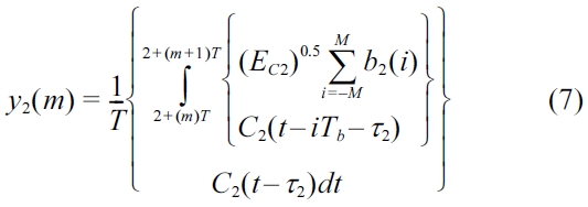
After performing integration over the given interval, we obtain the following results with the noise components as well as the cross correlation of signature waveforms.
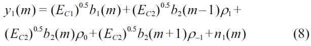
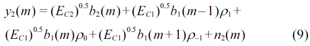
where coefficients
These symbols can now be decoded using an ML Viterbi decision algorithm. Viterbi algorithm can be used to detect these signals in much the same way as convolution codes. This algorithm makes a decision over a finite window of sampling instants rather than waiting for all the data to be received [1]. The above derivation can be extended from two users to K number of users. The number of operations performed in the Viterbi algorithm is proportional to the number of decision states, and the number of decision states is exponential with respect to the total number of users. The asymptotic computational complexity of this algorithm can be approximated as:
According to original Verdu’s algorithm [5], the outputs of the matched filter
follows:
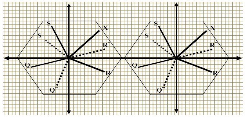
In addition, if vectors are regarded as points in a Kdimensional space, then the vectors constitute the constellation diagram that has K total points. This constellation diagram can be mathematically expressed as: ?= {T
Fig. 3 illustrates the constellation diagram that consists of three different vectors (lines) with the original vector ‘X’ that represents the collective complexity of the receiver.
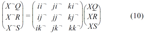
Equation (10) represents the following:
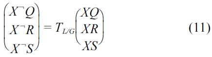
Equation (11) can also be written as:
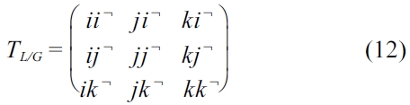
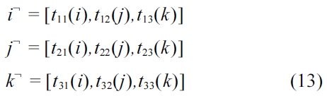
In Equation (12), the dot products of the unit vectors for the two reference points are in fact the same as the unit vectors of the inverse transformation matrix of (11). We need to compute the locations of the actual transformation points described in Equations (11) and (12). Let the unit vectors for the local reference point be:
Since,
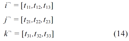
By substituting the values of
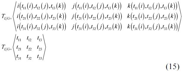
Substituting
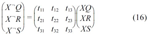
Equation (16) corresponds to the following standard equation used for computing the computational complexity at the receiving end: ?= {Tb} b ∈ {-1, +1}
This composition can be used to derive the collective computational complexity at the receiving end using (16). Since the channel is assumed to be LTI, the transformation points may occur in any coordinate of the constellation diagram. The positive and negative coordinates of the constellation diagram do not make any difference for an LTI propagation channel. In addition, the transformation points should lie within the specified range of the system. Since we assumed that the transmitted signals are modulated using BPSK which can at most use 1 bit out of 2 bits (that is,
Using (16), a simple matrix addition of the received demodulated bits can be used to approximate the number of most correlated transformation points. The set of the transformation points correspond to the actual location within the transformation matrix as shown in (16).
>
C. Complexity of the PE Algorithm
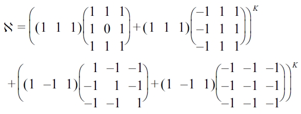
The entire procedure for computing the number of demodulated bits that need to be searched by the decision algorithm can be used to approximate the number of most correlated signals for any given set of transformation points. This is because, we need to check whether or not the transformation points are closest to either (+1, +1) or (-1, -1). The decision regions or the coordinates where the transformation points lie for (+1, +1) and (-1, -1) are simply the corresponding transformation matrixes that store the patterns of their occurrences. If the transformation points do not exist in the region (coordinate) of either (+1, +1) or (-1, -1), then it is just a matter of checking whether the transformation points are closest to (+1, -1) or to (-1, +1). In other words, the second matrix on the right hand side of (16) requires a comprehensive search of at most 5
The minimum search performed by the decision algorithm is conducted if the transformation points exist within the incorrect region. Since the minimum search saves computation by one degree, the decision algorithm has to search at least 4
Since most of the decisions are correct, we can reduce the number of computations by only using the transformation matrixes on those coordinates that are most likely to lead to an incorrect decision. By doing this, we greatly reduce the unnecessary processing required to make a decision regarding the correct region or the coordinate. Thus, the number of received demodulated bits that need to be searched can be approximated as: 5
The computational complexity of any multiuser receiver can be quantified by its time complexity per bit [14]. The collective computational complexity of the proposed PE algorithm is achieved after performing the transformation matrix sum using the complex properties of the existing inverse matrix algorithms. In other words, the computational complexity can be computed by determining the number of operations required by the receiver to detect and demodulate the transmitted information divided by the total number of demodulated bits. Therefore, both quantities T and b from our fundamental equation can be computed together and the generation forall the values of demodulated received bits b can be done through the sum of the actual T that approximately takes
Once the BPSK modulated bits (
>
D. Mathematical Proofs for Computational Complexity
This section provides the formal mathematical proof of the above discussion that proves the efficiency of the proposed algorithm with given input sizes. We provide a mathematical proof for both the upper bound and the lower bound of the proposed algorithm over the ND and the ML algorithms.
For the sake of this proof, we consider that each algorithm is represented by the growth of a function as follows: Let
Equation (17) shows that the proposed algorithm
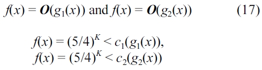
Solving for


Solving for
Thus, this is proved using (18). It should be noted that the
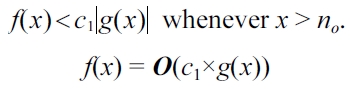
f(x) is said to be O(c2×g2(x)),
if and only if there exists a constant
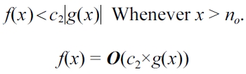
Thus, this is proved using (19).
To analyze the lower bound, we provide a proof in the reverse order to define a lower bound for the function
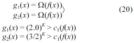
Solving for
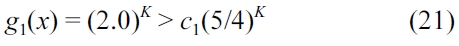
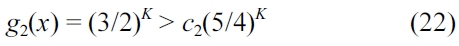
Solving for
g1(x) is said to be Ω(c1×f(x)),
if and only if there exists a constant
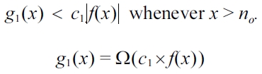
Thus, this is proved using (21). Solving for
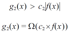
Thus, this is proved using (22). As we have proved here (referring (17) and (20)) that:
f(x) = O(c×g(x)) and g(x) = Ω(c×f(x))
IV. Performance Analysis of the PE Algorithm
The order of growth of a function is an important criterion for proving the complexity and efficiency of an algorithm. It provides simple characterization of the algorithm’s efficiency and also allows us to compare the relative performance of algorithms with given input sizes. In this section, numerical analysis is performed to observe the computational complexity of the proposed algorithm. Simulations are conducted in MATLAB (MathWorks, Natick, MA, USA) to evaluate the BER performance of a time-invariant DS-CDMA linear synchronous system in an additive white Gaussian noise (AWGN) channel. The original computational complexity of the ML optimal receiver is (2)
>
A. Analysis of Computational Complexity
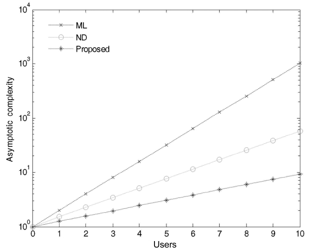
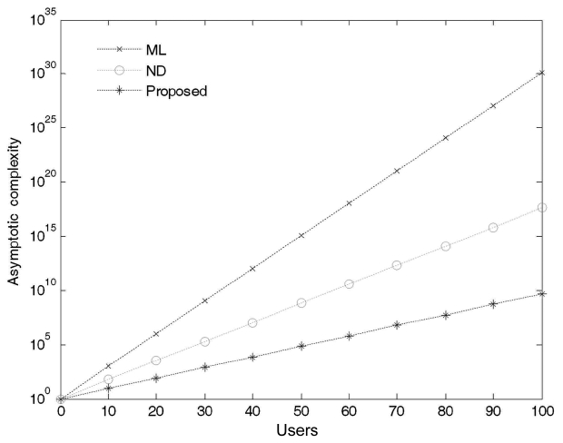
According to our numerical results, we successfully reduced the computational complexity at an acceptable BER after considering the DS-CDMA synchronous LTI system. The numerical results show the computational complexities with respect to the number of users as shown in Figs. 4 and 5 for 10 and 100 users, respectively. As the number of users increases in the system, the computational complexity differences among the three approaches become obvious.
Fig. 4 presents the computational complexities for a network that consists of 10 users. As we can see, the proposed algorithm for a small network of 10 users requires fewer computations as compared to the ML and the ND algorithms. In addition, the proposed algorithm greatly reduces the unnecessary computations involved in signal detection by storing the pattern of occurrence of the demodulated bits in the transformation matrix and uses it only on those coordinates or decision regions which are most likely lead to an incorrect decision. The computational complexity for a network that consists of 100 users is shown in Fig. 5.
It should be noted that the computational complexity curve for the proposed algorithm is growing in a linear order rather than in an exponential order. The computational linearity of the proposed PE algorithm comes at the cost of not considering all the decision variables and thus provides much better performance over the ND and the ML algorithms. In other words, this can be considered as an extension of the former results that demonstrate the consistency in the linear growth for the required computations of the proposed algorithm. As we increase the number of users in the system, additional transformation matrixes will be used to determine which coordinate(s) or
decision region(s) within the constellation diagram is most likely to produce errors.
>
B. Performance Analysis of BER Performance
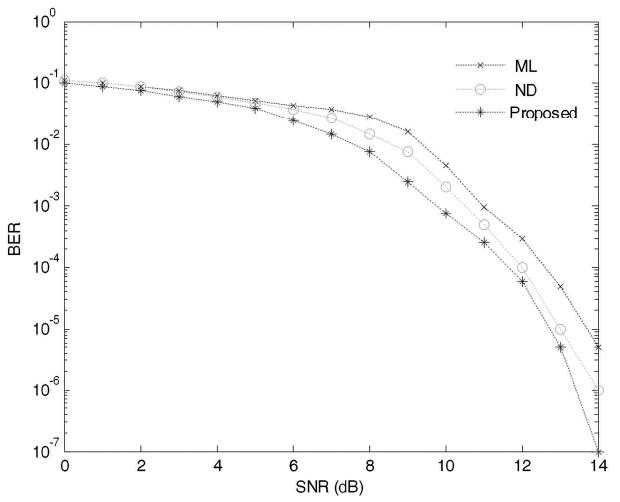
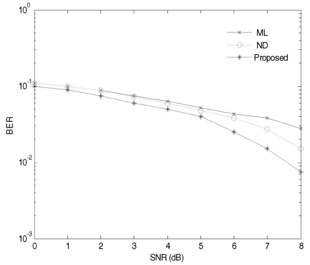
Simulation results show that the proposed technique performs better than the ML and the ND algorithms for all values of BER. Figs. 6 and 7 display a plot of three BER versus SNR curves. These curves were plotted in an AWGN channel for a small range of users. It should be noted that the BER performance of the proposed technique is always better than the ML and the ND algorithms as shown in Fig. 6. For the first few values of SNR, the ND algorithm nearly approaches the ML algorithm whereas the proposed technique still maintains a reasonable performance difference. It can be seen in Fig. 6 that the proposed technique achieves less than 10-2 BER for SNR = 8 dB which is quite close to the required reasonable BER performance for a voice communication system. For small values of SNR, the BER for these three algorithms is almost equal, but as we increase the value of SNR, typically more than 10 dB, one can clearly observe the difference in the BER performance.
The former result demonstrates a slight improvement over the BER performance shown in Fig. 6 for all SNR values above 9 dB. Even for small values of SNR, the proposed technique demonstrates better performance than the ML and the ND algorithms. As the value of SNR increases, the BER performance of the proposed technique over the ND and the ML algorithms becomes more and more substantial because the probability of having more divergent values of SNR increases. It can also be noticed in Fig. 7 that the proposed algorithm achieves
less than 10-3 BER for SNR = 10 dB, which is more than what we desire for a voice communication system. Furthermore, the proposed technique achieves 10-7 BER performance for SNR = 14 dB as shown in Fig. 7. This is more than an acceptable value of BER for data communication such as file transfer protocol (FTP) and is quite close to the desired value of BER (typically 10-8 BER is required) for high fidelity digital audio systems.
In this paper, we presented a new PE algorithm that utilizes the transformation matrix scheme to improve the performance of next generation wireless receivers. This paper provided an implementation of the proposed PE algorithm with the support of a well driven mathematical model. To prove the low-complexity and the correctness of the PE algorithm, we provided a formal mathematical proof for both the upper and lower bounds of the algorithm. The mathematical proofs for both bounds demonstrated that the complexity of the proposed PE algorithm with any input size is always less than the ML and ND algorithms. The reduction in complexity increases the computing power of a multiuser receiver. Consequently, the increase in computing power would likely result in fast signal detection and error estimation which do not come at the expense of performance. Even though the proposed algorithm requires fewer computations for signal estimation and detection, the practicality of our method and the expected results depend on a realistic system model. For the sake of implementation regarding our proposed algorithm, a more practical asynchronous system would be considered in the future that consists of non-linear time variant properties of the Gaussian channel with an imperfect power control. Specifically, we will extend the proposed approach for CDMA based non-linear likelihood multiuser detectors for the following conditions: wireless multipath fading channels, known and unknown multiple access interference, broadband data, and power control variations.