Emerging systems with multi-core chips, high-density blades, and sometimes specially designed accelerators including graphics processing units (GPUs) have the potential to provide much higher capacity and capability for scientific computational research than previous generation systems. While this unprecedented scale of computational resources has become relatively accessible for most of the science and engineering community, it is a well-known fact that only a small fraction of the theoretical peak performance of these systems is obtainable for the vast majority of high performance computing (HPC) applications [1]. Challenges for achieving optimized performance and better scalability exist in almost all aspects of HPC system utilization.
In this study, the development and analysis of computational methods on performance optimization and scalability for two class-representative scientific codes has been successfully conducted on world-class HPC systems. Basic optimizations have implemented to enhance on-node performance, and a series of tests for improving scalability followed. Throughout this study, many of the critical insights and knowledge gained will be a useful guideline for the future development of large-scale HPC applications aiming to improve performance. In the optimization, a new performance tool, PerfExpert [2], developed by Texas Advanced Computing Center (TACC) and the Computer Science Department at The University of Texas at Austin, was used. The development goal of PerfExpert was to provide an easy-to-understand interface for users and step-by-step guidance for optimization. By utilizing this tool it was possible to maintain a unified structure of performance test outputs for many different cases. Most of performance and scalability tune-ups in this study are based on the results from the PerfExpert.
Overall, the knowledge gained from this study is applicable to other real-world scientific HPC applications optimization and will also provide users with insights into the performance engineering of large-scale application development.
There are many factors that affect the performance and scalability of applications when going to large core counts on an HPC system, both at the node level and across the whole system. A systematic approach was taken in this study to analyze these issues and to apply suitable techniques for the performance improvement and scalability of the selected benchmarking applications, as described in the rest of this report. A small-scale, three-dimensional (3D) heat transfer code and a lattice-Boltzmann multiphase (LBM) simulation code have been selected. The heat transfer code is written in a way that can demonstrate various performance benchmarks, and has been used in numerous tutorials and workshops for educational purposes. The LBM code serves as a real-world scientific model example.
In general, baseline study for application optimization starts with profiling. This step includes node level performance diagnostics and analysis, and investigation on applicable optimizations for selected applications. Based on the results from the profiling, the next step is comprised of numerous optimizations with algorithm development and implementation, followed by code validation and test-drive for scalability. In this study, we categorize the optimizations into four different groups:
Intra-node performance optimization: TACC has been conducting research on node-level performance optimization and the development of performance diagnosis tools in collaboration with the Computer Science Department at The University of Texas at Austin. PerfExpert, an easy-to-use node-level performance diagnosis tool that is developed through that collaborative effort, has been used in order to ensure the application achieves maximum performance within a single node.
Inter-node performance optimization: Methods for increasing scalability across the system will include algorithm and software scaling. A hardware scaling study was excluded as it lies beyond the boundaries of this project. Profiling and communication analysis was the focus of the investigation on inter-node optimization. Timing and structural studies of the message passing interface (MPI) layer used in the application codes were carried out, and changes were implemented in order to improve the initial scaling by minimizing overhead, bottlenecks and workload imbalance from the codes.
Hybrid programming for scalability: An attempt was made to optimize the use of node-level memory resources by modifying the applications to include OpenMP statements. This may also be of benefit for overall scaling because of reduced communication traffic over the network, and increased bandwidth available to the tasks carrying out the MPI exchanges. Intra-node performance evaluation as well as overall scaling were analyzed again and compared critically to those of the original, pure MPI applications.
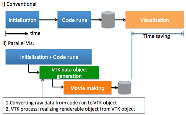
Real-time, in-situ parallel visualization: In addition to code implementation, extra effort in developing an insitu parallel visualization plug-in was made. By implementing this plug-in, users can have visualization toolkit (VTK)-compatible binary objects in their hands at the end of computation runs, and the binary files are easily converted into animation by visualization tools such as ParaView and VisIt. This addition improves overall productivity of the modeling cycle by reducing the post-process time.
In Sections III and IV, computational methods used in the optimizations study are described in detail.
III. OPTIMIZATION OF A CONVENTIONAL POISSON SOLVER
>
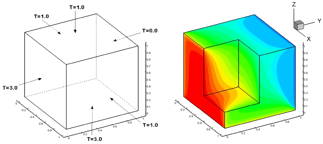
A. 3D Conductive Heat Transfer Code
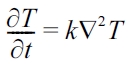
The heat transfer code (called Heat3D) solves the heat conduction partial differential equation shown below by using the tri-diagonal matrix algorithm (TDMA). Fig. 1 presents the description of computational mesh with the boundary condition and what the code simulates.
The code is written in Fortran90 and is parallelized
with MPI. 3D domain decomposition in Cartesian coordination has been utilized for scalability. In a previous study [3], the model has thoroughly been tested for various test cases of 1D, 2D, and 3D domain decomposition along with multiple cases of communication schemes. The current version for this study is implemented with MPI virtual topology for 3D decomposition, and also is utilizing user-defined MPI data types (contiguous, vector) for better data packaging and more efficient communication. Since this code was developed for educational purposes in performance benchmark and optimization, it is a great exemplary application model for baseline study. Users can control all aspects of calculation and are also able to measure details of communication work. Base output from the code is time measurements of computation vs. communication work. The times are measured by MPI-default MPI_WTIME, and this setup invokes communication overhead from a multiple synchronization barrier.
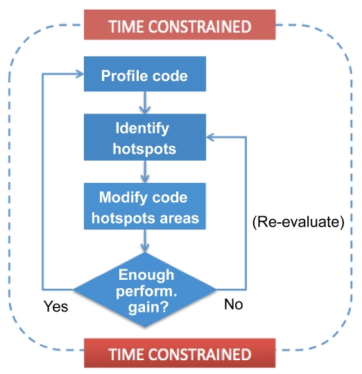
On-node performance optimization starts with application profiling. By using multiple profiling tools, users are able to identify the bottleneck of the code performance and apply available optimizations to those bottlenecks. Fig. 2 briefly illustrates the general optimization steps. While this looks straightforward, critical aspect of this process is how to interpret those performance data generated by profiling tools.
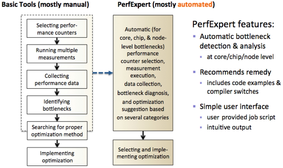
To make performance optimization more accessible, TACC and the Computer Science Department at University of Texas at Austin have designed and implemented PerfExpert, a tool that captures and uses the architectural, system software and compiler knowledge necessary for effective performance bottleneck diagnosis [2]. Hidden from the user, PerfExpert employs the existing performance tool, HPCToolkit [4], to execute a structured seq-
uence of performance counter measurements. Then, it analyzes the results of these measurements and computes performance metrics to identify potential bottlenecks at the granularity of six categories. For the identified bottlenecks in each key code section, PerfExpert’s built-in component, Autoscope, recommends a list of possible optimizations, including code examples and compiler switches [5].
In summary, PerfExpert is an expert system for automatically identifying and characterizing intrachip and intranode performance bottlenecks and suggesting solutions to alleviate the bottlenecks. Fig. 3 displays the comparison between the manual optimization process and PerfExpert utilization.
PerfExpert was utilized thoroughly in this study, giving a unified, structured way of analysis regarding application performance. Another light-weight tool used for
analyzing MPI-related performance is mpiP [6] developed at the Lawrence Livermore National Laboratory (LLNL).
As expected, the on-node performance evaluation of the Heat3D code started with the PerfExpert test. First, what PerfExpert tells you (shown below) is that the TDMA routine in the code is spending more than 86% of the total runtime, suggesting that we need to focus on this routine since the other routines all together are taking less than 15% of the total runtime. This is a typical example of the computationally intensive numerical model. Communication overhead of this model is around 15?20%, which remains consistent throughout the test, which will be described in a later section with mpiP test results.
First test case is 2563 mesh size with 8 cores (2×2×2 decomposition: 1283 per core).
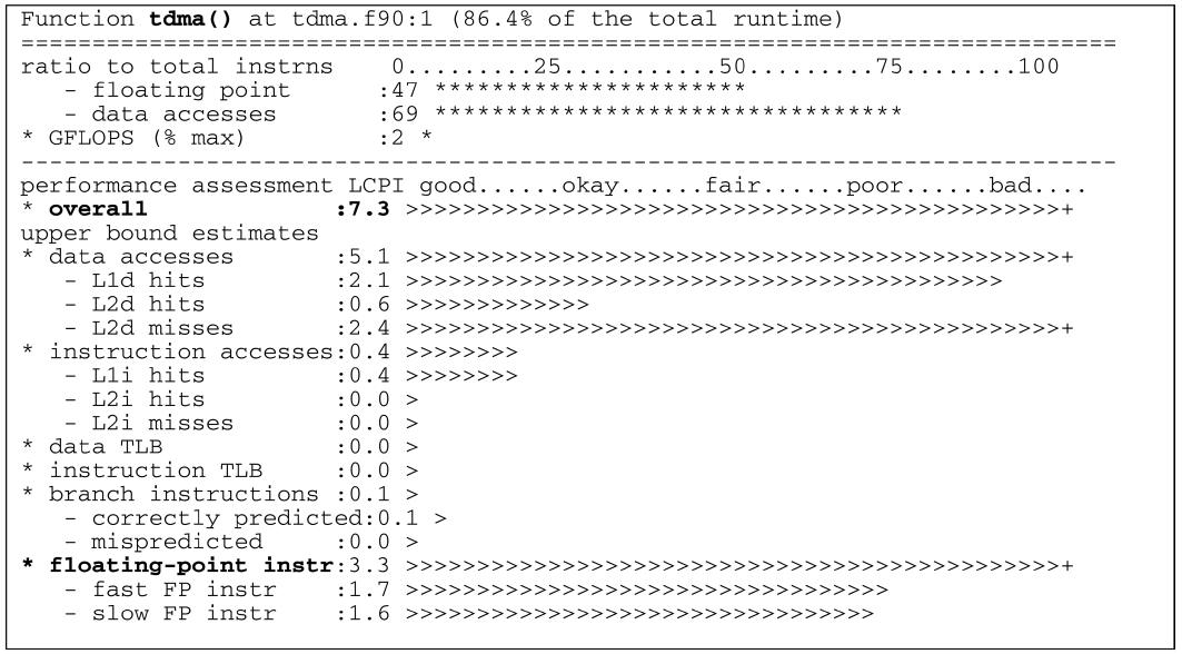
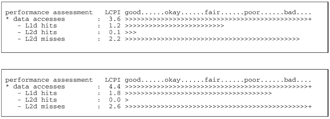
As shown in the profiling result with PerfExpert, the TDMA routine in the Heat3D code has a major issue in data access and floating point operation. The problem with data access is not a surprise since the TDMA solver in the code has multi-dimensional array calculations within multiple loops. The floating point instruction is a little tricky as the long bar could mean the computationally intensive aspect of the code. Optimization in the memory access pattern of the code can put more work on the computation, which will increase the local cycles per instruction (LCPI) number for floating point instruction, and it indicates the code runs more efficiently.
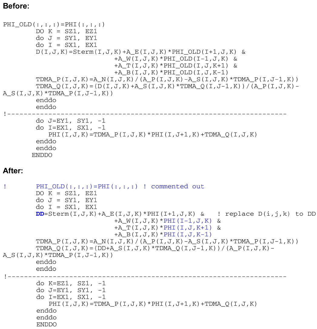
The first optimization for the code is replacing the array with a scalar value, therefore reducing the required memory footprint, and increasing the effectiveness of the memory access pattern. Within the TDMA routine, an array D(i,j,k) can be replaced to a scalar variable since the value of D(i,j,k) at each grid point is unique and is independent of the values of any other grid points. By replacing the array to a scalar, the runtime of the code is reduced by almost 10% (from 295 seconds to 265 seconds for 2563 size with 8 cores: 1283/core size). The result from the second PerfExpert run after the optimization is shown below. The results show that the overall LCPI value for the TDMA routine is reduced to 7.0, and the floating point instruction LCPI value increases to 3.4. They are small changes in terms of local cycle instruction (LCI) value, but the actual runtime improves by 10%.
The second optimization scheme used is to reduce the redundant use of memory space. In the baseline version,
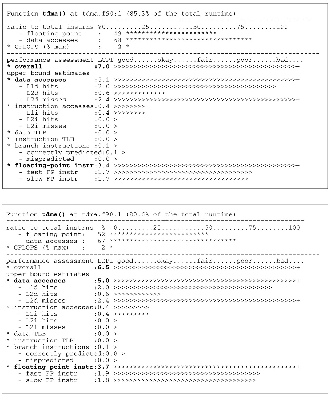
the variable PHI(i,j,k) used in main routines and the one used in TDMA routine, PHI_OLD(i,j,k), carry the same value until it is used in the triple loop calculation in TDMA. The different names in those routines are not necessary except that the different names illustrate the logical meaning of it at different time steps, but the actual values are the same. By replacing PHI_OLD with PHI and using the same array without creating another duplicated one, the memory access obtains greater efficiency than the previous version. Actual test results showed this optimization reduces the runtime from 265 to 235 seconds, which is more than 10%. Next the updated result from the PerfExpert test shows that overall and data access LCPI values are decreasing while the floating point instruction LCPI value increases to 3.7.
Below the code section of before and after of the optimization is shown. The lines highlighted with blue color are where changes were made for optimization.
Although other optimizations are still possible, we shift our focus on to inter-node scalability as the main goal of this study is to provide general computational approaches to scalability for large-scale applications.
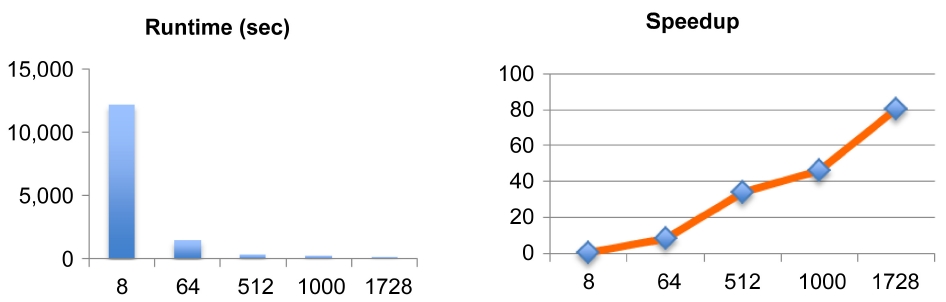
For scalability of application in the HPC environment, the first test to be done is the strong scalability test. By increasing the number of processors (cores) for the same problem size, it is possible to identify the sweet spot of parallel efficiency. At the same time, the speedup graph also helps to understand what number of cores is the most
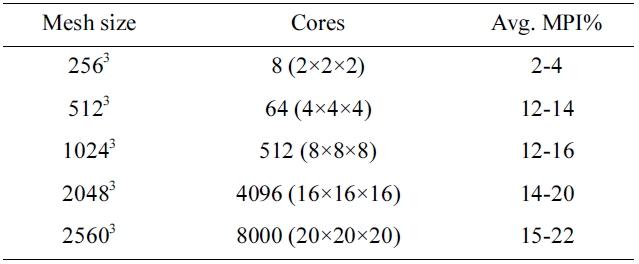
[Table 1.] Cases for weak scaling test of Heat3D code

Cases for weak scaling test of Heat3D code
efficient for a certain size of a given problem.
Fig. 4 demonstrates the speedup of the Heat3D code of 10243 mesh size with increasing the number of cores. Please note that it is not compared against serial run as the problem size is too big to have a reasonable runtime. Though its not linear, the plot shows a good scalability of the code. The limitation of this test is the available memory size on a single node, as the size of the problem cannot be larger than 10243 mesh due to the maximum
memory limit per compute node of the system. This is usually the first hurdle when application developers want to scale up their parallel code. Since most of parallel codes are evolved from a serial version, often times the mesh generation part is coded for using a global memory space rather than a distributed memory type for MPI parallelization.
The Heat3D code is updated with a parallel mesh generation feature for this study and the upgraded model is now capable of running much larger problem sizes. Table 1 shows the test cases for weak scaling of the parallel mesh version of the Heat3D code. By sustaining the sub-mesh size per single core to 1283, and with an N3 domain decomposition scheme, it was possible to increase the problem size up to 25603. This is more than 8 times bigger than the previously limited size of 10243. It was possible to increase the size even more, but the test was done at this size because of the number of cores involved.
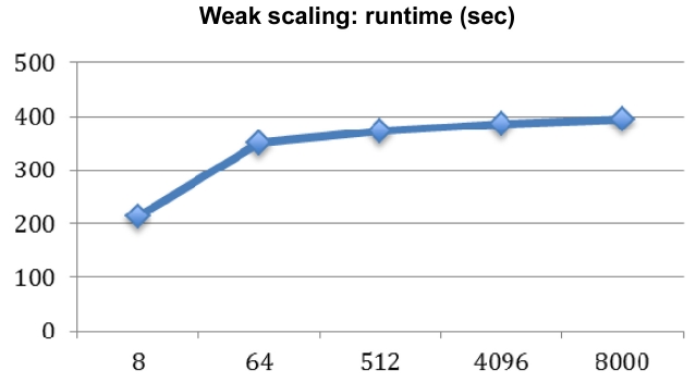
Fig. 5 shows the result of weak scaling, and the runtime (second) of increasing the problem size with a fixed number of cores remains fairly consistent after a big jump in the initial stage between 8 to 64. We believe this jump is due to the initial job launching time of the Mvapich MPI stack through the InfiniBand (IB) switch when it handles multiple node job launching.
>
D. Hybrid (MPI+OpenMP) Model
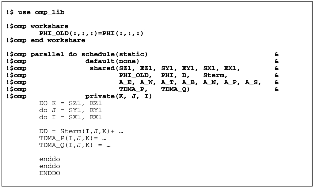
Even when the parallel mesh version of the fairly welloptimized code hits a scalability limit, one strategy that addresses an even larger problem size is to go with hybrid programming. Many researchers consider using this strategy to boost the performance of their numerical models; however, in reality, the hybrid programming approach does not guarantee performance improvement. On the other hand, by setting MPI processes with muti-threaded OpenMP tasks, it is possible to reduce the memory footprint per node; hence a much bigger problem size can be addressed. The Heat3D code is an ideal case for hybrid programming as more than 80% of the total runtime is spent in one computational routine, therefore implementing OpenMP muti-threads for the main computing routine will scale up the problem size while taking a minimal performance penalty. Below is the code snippet of the TDMA routine that features OpenMP implementation in the main calculation loop. For every iteration, this triple loop calculation will now spawn out multiple threads for parallel tasks depending on the number of thread users set up per MPI process.
>
E. Real-Time, In-Situ Parallel Visualization
While much of the work in this study focuses on code optimization and scalability for the computation process, post-processing (data management and visualization) is also a great candidate for increasing the productivity of computing workflow. Computational scientists these days are generating an unprecedented scale of data every day, and many of them are still using a manual post-processing script, or still trying to visualize their data with a less capable visualization tool. In this study, we developed a VTK-compatible plug-in for a Heat3D code in order to enable the visualization process in parallel while the computation is still running. Development of C++ routine that creates VTK objects is somewhat straightforward, but converting ASCII data generated by the Fortran Heat3D code into a C-compatible binary was tricky. Due to the difference of memory access pattern and indexing, the TACC visualization staff had to work with the code line by line. Naturally, developing a generic framework for the same purpose would be the next step, but in this study, development of a customized plug-in for the Heat3D code was sufficient. Adding extra VTK functionality of generating an animation movie so that application developers can have the final product of their computation at the end of the run is the plan for the next stage. Fig. 6 illustrates the mechanism of the real-time, parallel in-situ visualization process.
IV. OPTIMIZATION OF LATTICE-BOLTZMAN MULTIPHASE SIMULATION MODEL
When investigating the classes of scientific codes that should be considered for a comprehensive applicationbased benchmark there are several options that can cover particle-based methods, including molecular dynamics (MD) and the lattice Boltzmann method (LBM). The LBM has a simpler message passing structure than MD, because the number of messages exchanged between neighboring tasks is typically known in advance, and from a computa-
tional point of view the structure and behavior of an LBM code is similar to that of an MD code:
1. Calculation of local quantities for each “particle”
2. Particle displacement
3. Calculation of global, macroscopic quantities which affect the dynamics
4. Repeat 1?3 for a set number of time steps.
This suggests that an LBM code is a good starting point for this class of applications because it has most of the structural characteristics of other particle-based methods but it also has a straightforward implementation.
Although a simple single fluid LBM code is more straightforward to implement and analyze, we have chosen a multiphase flow LBM code as one of the two working codes for this project. One of the principal reasons for this choice is that a multiphase flow LBM code requires the calculation of gradients, Laplacians, and other differential quantities that are commonly required also in other scientific particle-based codes. This makes the use of this code as part of a comprehensive suite of benchmark applications more realistic. Also, a multiphase code deals with many more variables and arrays than a single fluid code and presents more opportunities for analysis and optimization.
One of the most challenging issues in the study of multiphase flows is the range of spatial and temporal scales that need to be analyzed. Interfacial phenomena can be localized in small volumes, but for the models to be useful the calculations often need to extend far beyond the interfacial regions. Also, the timescales involved in interfacial phenomena are short, but at the same time one needs to be able to simulate the evolution of the multiphase system over significant periods of time.
Traditional computational fluid dynamics (CFD) methods are capable of large system evolution simulations, but tend to use high-level models to represent interactions at the interface level. Kinetic techniques like the LBM [7] are better suited to more detailed analysis of short time scale evolution, but are hindered by their explicit nature and require many time steps to produce useful results. Parallel implementations [8,9], adaptive meshing algorithms [10,11] and multiple meshing levels [12], have helped improve the performance of LBM so that more simulation steps can be taken per second, but large scale simulations over long periods of time remain a challenge.
This chapter describes the multiphase model implemented in this LBM benchmark. The physical equations that are simulated are the Navier-Stokes equation together with the mass conservation equation, and a convective Cahn-Hilliard equation to track the interface evolution:
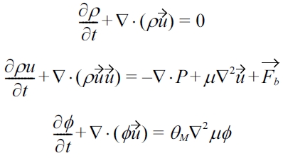
where
The Zheng-Shu-Chew model for two-phase flow [13] is limited to fluids with identical viscosity

Here Ω is the collision term in the Bhatnagar-Gross- Krook (BGK) [14] approximation:
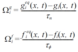
where
The macroscopic quantities corresponding to the order parameter
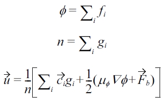
where
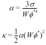
μφ=4α(φ3?φ*2φ)?κ∇2φ
with
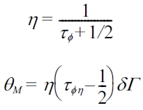
The expressions used for the relaxation parameter
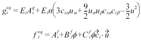
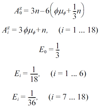
The equilibrium distribution functions are given by:
The
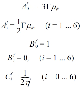
The
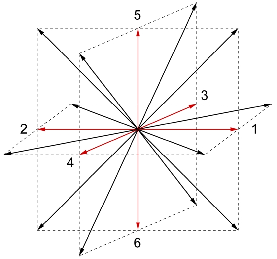
The velocity directions corresponding to these discretization schemes are shown in the figure below.
A basic implementation of the model described above has a simple structure:
1. Initialize f, g
2. Initiate the interface relaxation loop
a. Follow steps 4.a through 4.i without applying the gravity force
3. Complete the interface relaxation loop
4. Initiate the evolution loop
a. Update values of ρ, φ and u
b. Calculate chemical potential using the gradients and Laplacian of φ
c. Calculate interfacial forces using the chemical potential values
d. Perform collision step
e. Use MPI exchanges to get outward pointing f values on task boundaries
f. Stream f and g values along velocity directions
g. Use MPI exchanges to update inward pointing f and g values on task boundary nodes
h. Apply boundary condition modifications
i. Use MPI exchange to update φ values on task boundaries
5. Complete evolution loop and save data
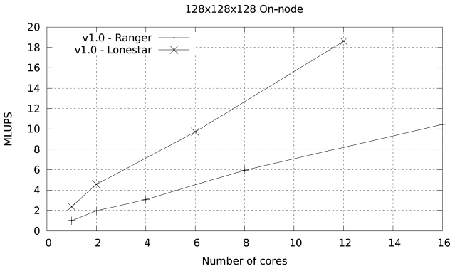
The performance of this basic implementation on a single node is illustrated in Fig. 8. The code (given as version 1) achieves a maximum of 10.44 millions of lattice updated points per second (MLUPS) when executed on a single Ranger node (16 cores of 2.2 GHz Opteron CPUs), and 18.61 MLUPS on a single Lonestar node (12 cores of 3.3 GHZ Westmere CPUs). The difference is larger than what one would expect from the shear clock speed difference between the two systems (50%) because this code is memory-bandwidth limited, and the Westmere system has a larger bandwidth per core than the Opteron system (2 GB/sec per core vs. 1.25 GB/sec).
>
B. Reuse of Intermediate Results
Analysis of this code by both PerfExpert and another performance profiling team, TAU, indicates that the code would benefit from reusing intermediate results. When looking at the structure of the code for version 1 a possible way to reuse intermediate results seems obvious: to combine the updates of
Because of the data dependencies, the value of
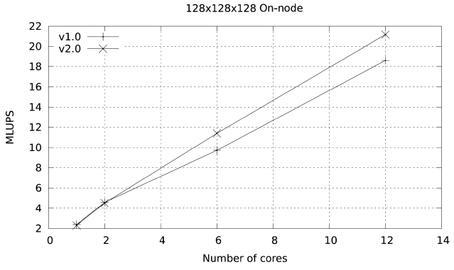
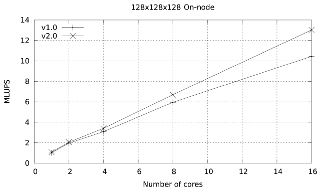
Figs. 9 and 10 illustrate the on-node performance of versions 1.0 and 2.0 of the code. The improvement in
performance becomes more obvious as more cores are used in the calculation. This is because the optimizations made so far focus on memory access, and become more
obvious as the number of cores per node participating in the calculation increases and the memory bandwidth per core is reduced.
>
C. Arithmetic Simplification and Reduction of Memory Accesses
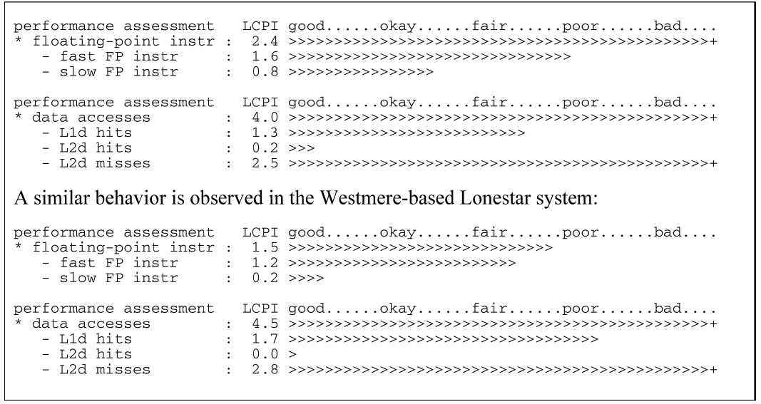
Further analysis of version 2 of the code suggests that there is room for improvement in the area of floating point operations. In particular, when run on the Ranger architecture, this version of the code has a full third of the floating point operations being what PerfExpert classifies as “slow” floating point operations:
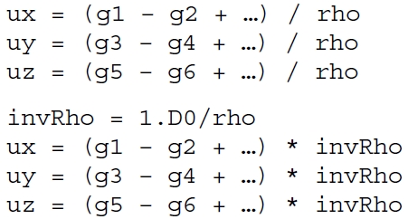
In order to improve this we focused on the function collision, which both PerfExpert and Tau indicated was the most time-consuming subroutine in the code. We defined several inverse values so that we could turn multiple divisions into a single division and multiple products as in:
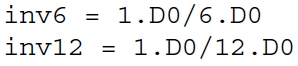
We also defined a series of inverse values for constants used in the gradient and Laplacian calculations:
We also manually re-arranged the terms in the equilibrium function calculation and the collision step to minimize the number of floating point operations, and in particular to reuse as much data as possible by defining some terms which are common to all the principal directions, and some terms which are common to all diagonal directions. This also reduces the number of memory accesses, which is another weak area highlighted by both PerfExpert and Tau.
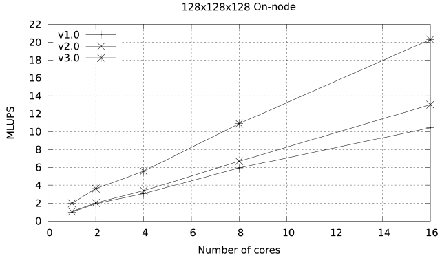
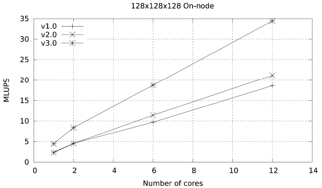
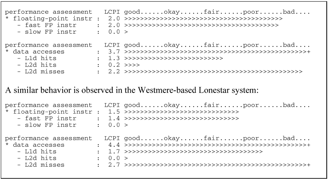
The result from these changes is version 3 of the code, with a performance of 20.31 MLUPS on a single Ranger node and 34.44 MLUPS in a single Lonestar node. This improvement in performance is shown in Figs. 11 and 12, and is also seen in the output from PerfExpert in the Ranger system.
Not only do these changes reduce the number of floating point operations per second (FLOPS) needed by 20%, but they virtually eliminate the presence of slow floating point operations. The changes also reduce the number of L2 cache misses by almost 14% and the overall data accesses by 8%. Further improvement in the memory access patterns of this particular code may be possible but it is not obvious, since the streaming step in LBM makes contiguous access very difficult. This takes us to a performance close to 15% of peak in Lonestar, and at this point we consider the possible improvements to the scalability
of the code.
>
D. Memory Access Improvement in Data Packing and Unpacking
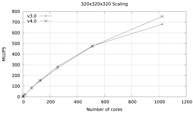
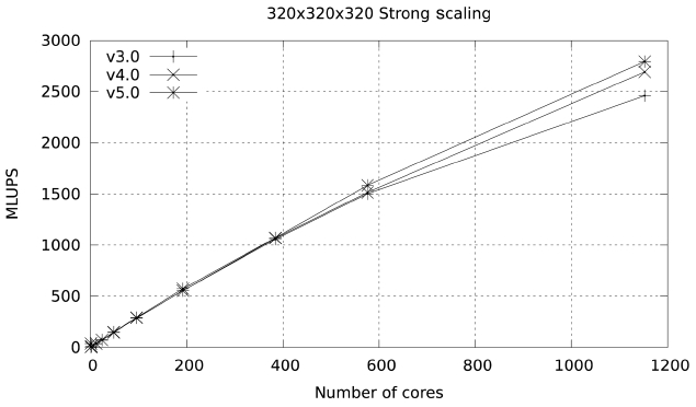
Versions 1?3 of the code use a fat loop in order to pack the data that is needed in the MPI exchange. This loop involves multiple arrays and multiple non-contiguous locations within the arrays. Since both PerfExpert and Tau indicate a very large percentage of cache misses in the MPI exchange routines poststream.f90 and postcollision. f90 the next step in the optimization of the code was to split this loop into shorter loops involving a single array with the hope that prefetching, and with it the scalability of the code, and with this change, the scalability of the code will be improved.
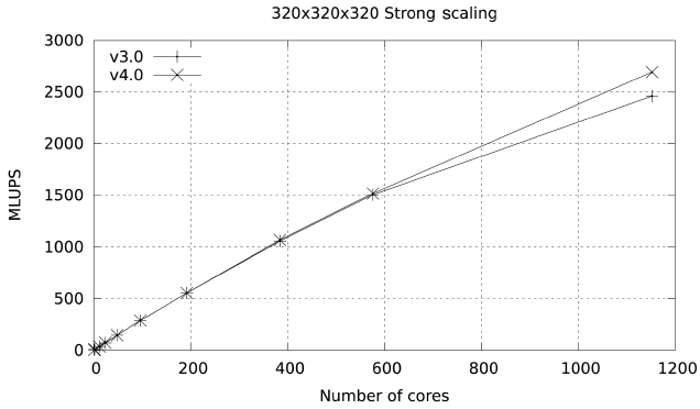
The results of this simple change are highlighted in Figs. 13 and 14. At 1024 cores the parallel efficiency of version 4 in Ranger is 5% higher than the efficiency of version 3, and the improvement in Lonestar at 1152 cores is close to 4%. PerfExpert shows a tiny reduction in over-
all data access timings which corresponds to these changes:
We also observe a lo-wer amount of time spent in L2 cache misses in the Westmere-based system.
By using loop fission and simplifying the memory access patterns in the data packing and unpacking sections of the MPI exchange subroutines we have improved the scalability of the code but in the process it also became obvious that such a large amount of data packing/ unpacking would benefit from using fully non-blocking communications so that part of this data packing and unpacking process can be overlapped with the message passing itself.
>
E. Overlapping Computation and Communication
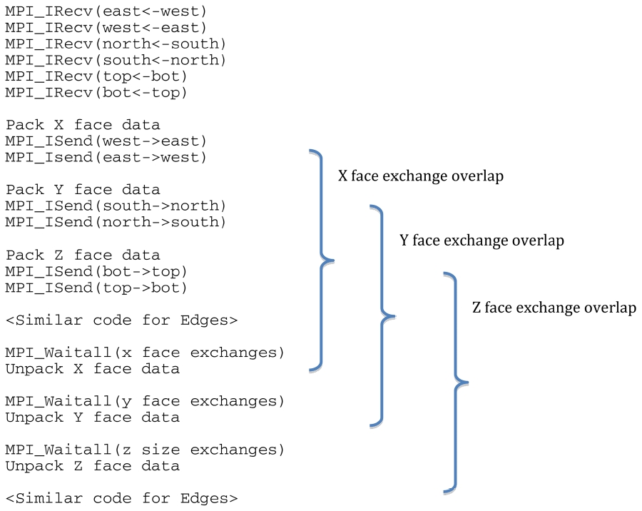
In version 5 of the code all data exchanges are done using MPI_Irecv/MPI_Isend calls followed by a single MPI_Waitall statement just before that data is needed for unpacking.
To obtain maximum overlap we defined several sets of messages that were completed with a single MPI_Waitall statement, one for each of the face exchanges in the X, Y, and Z directions, and one for each of the edge exchanges in the X, Y, and Z directions. In this manner part of the data exchange for the faces in the X directions can be partly overlapped with the packing of data for the Y and
Z exchanges, the Y exchange can be partly overlapped with the packing of data for the faces in the Z direction and the unpacking of data corresponding to the face exchange in the X direction, and so on and so forth. The pseudo code of this would read.
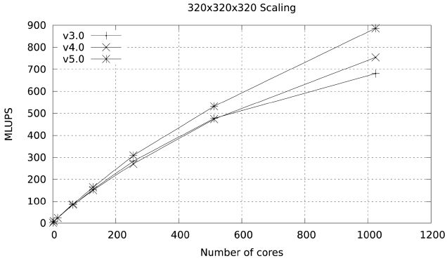
These changes produce a very marked improvement in scalability, increasing parallel efficiency to 60% at 1024 cores in Ranger and to 76.9% at 1152 cores in Lonestar.
Figs. 15 and 16 illustrate this improvement.
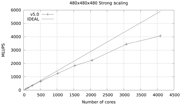
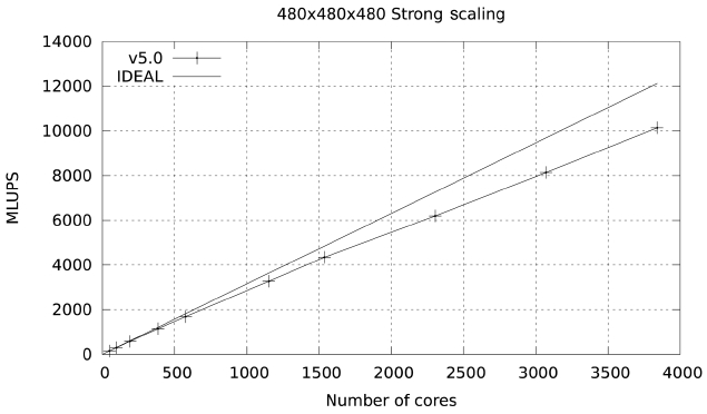
Studies were also carried out with a large data set (480×480×480), with a footprint of approximately 36 GB in memory. The results for both Ranger and Lonestar are shown in Figs. 17 and 18. In these figures some fluctuations in performance (which are repeatable) are observed. These fluctuations are due to the particular partitioning scheme chosen for the spatial decomposition of the problem. The large difference in parallel efficiency between the runs in the two systems occurs because the MPI part of the code is dominated by the exchange of large messages, so that the scalability of this code is limited by network bandwidth. The increased network bandwidth provided by the quad data rate (QDR) IB in Lonestar (40
GBs) over the 10 GBs SDR IB of Ranger explains the difference.
Study on computational methods for on-node optimization and inter-node scalability for HPC applications has been conducted. By using a newly developed performance diagnosis tool, PerfExpert, a basic guideline of on-node optimization was developed for two selected scientific applications. An algorithmic approach for improving scalability was also introduced and tested with a large number of cores on HPC systems.
The methods developed in this study can be used for future research on application-based benchmarks. PerfExpert proved its capability of providing appropriate optimization guidelines as each test case showed performance improvement. Multiple case studies on scalability were also provided, including MPI data packaging, utilizing MPI non-blocking communication for overlapping computation and communication, and hybrid programming with MPI and OpenMP. In addition, VTK-compatible in-situ visualization plug-in was developed as well to provide a way of enhancing the effectiveness of the overall modeling workflow.
During the course of this project, it has been apparent that more research will be required for more extensive guidelines regarding optimization and scalability. Additional case studies with more applications from various science domains are necessary if a general framework for an optimization process in high demand.
The next stage of this project will include a similar study on new HPC platforms such as general purpose computing on graphics processing units (GPGPU) and Intel’s upcoming many-integrated core (MIC) system. As many HPC researchers expect the development of new parallel programming models for those new platforms, this study provides application developers with a stepping stone in developing new computational methods for HPC applications.