Serious environmental concerns and increasing energy costs have placed emphasis on the need to develop sustainable renewable energies. The use of renewable energies such as biomass, wind, solar energies, etc helps us to diminish the heavy reliance on fossil fuels[1]. As one of renewable clean energy sources, biomass has been extensively studied with the focus placed on the conversion of biomass into biofuels. A variety of energy needs such as electricity and fuels can be covered by biomass because of its availability and its environmental benefits. In addition, it can be used for other industrial purposes such as the production of various biochemicals[1].

The industrial use of various biomass resources for the production of biofuels requires rapid characterization of their chemical and physical properties. The most useful property in biofuels is the calorific value, which is affected by many factors such as moisture, ash content, and the chemical composition of biomass. Irregular or heterogeneous characteristics of biomass feedstocks make rapid and reliable assessment and prediction of their properties crucial for the production of bio-fuels. However, traditional laboratory analysis cannot be a solution due to its time consuming, expensive, and off-line nature[2].

As one of promising alternatives, near-infrared (NIR) spectroscopy approach has been successfully used in many industrial fields including biomass as well. NIR spectroscopy is preferred because of its non-invasive and informative characteristics[2]. Instead of off-line analysis of biomass by conventional laboratory approaches, the use of NIR enables us to determine essential quality parameters or properties of biomass in an on-line basis. On the other hand, NIR outperformed other popular spectroscopic techniques, for example infrared (IR) and Raman spectroscopy, in terms of minimum sample preparation required and real time responses[3].

Prediction of biomass properties using spectroscopic NIR data is a multivariate calibration problem, in which chemometric approaches have been used including principle component regression (PCR) and partial least squares (PLS). By applying these techniques to spectroscopic data, one can construct prediction models for biomass properties of interest because of the simplicity to build or use, accessibility, and speed. PLS and PCR are dimension reduction techniques that determine a set of latent variables by maximizing the covariance of two variables, i.e., predictor X of NIR spectra and response Y of biomass properties. Thus the relationship between NIR and biomass properties can be modeled by such prediction techniques. They have been shown to be useful in various calibration problems especially for high dimensional noisy data with collinearity[2,3].

Linear prediction techniques, however, may have some limitations when dealing with nonlinear data such as spectroscopic NIR data. Using linear prediction techniques may be misleading because nonlinearity of the data cannot be modeled appropriately. The selection of linear or nonlinear techniques depends on the characteristics of problem and data. Recently, nonlinear kernel methods such as kernel PLS (KPLS) and support vector regression (SVR) have been used to model nonlinear behavior of the data[4,5]. Basically, input raw data are first mapped into a kernel feature space by a nonlinear mapping function and then these mapped data are analyzed. Thus they have the ability to model nonlinear relations and lead to a global model to provide efficient handling of high dimensional data.

In this work, the applicability of nonlinear chemometric techniques based on biomass NIR spectra data is assessed for the rapid prediction of ash/char contents in different types of biomass. The prediction performances of both linear and nonlinear prediction models are compared using six types of biomass NIR data. These models seek to find patterns in NIR data that correlate with changes in biomass properties. Thus, prior to building prediction models, preprocessing of NIR spectra data is quite important. because noise or background information need to be reduced. The selection of appropriate preprocessing methods is also presented in terms of building robust prediction models with good predictive ability. This paper is organized as follows. Short reviews of linear and nonlinear techniques are given in section 2, and then biomass NIR spectra data and details about prediction results are presented along with the evaluation of preprocessing methods. Finally, concluding remarks are given.

Principal component analysis (PCA) seeks to find eigenvalues (λ ≥ 0) and the associated eigenvectors v satisfying

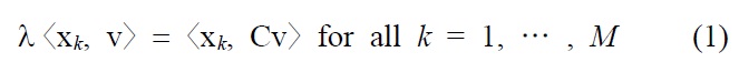
where C is the M sample estimate of the covariance matrix and 〈x_k, v〉is the dot product between x_k and v[6]. To model a relationship between independent variables X and dependent variable (s) Y, PLS method seeks to find weight vectors w and c that maximizes the sample covariance between t and u[8]. Here, t and u are score vectors for X and Y, respectively. By regressing X (Y) on t (u), a loading vector p (q) can be obtained as follows:

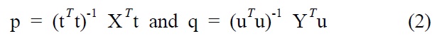
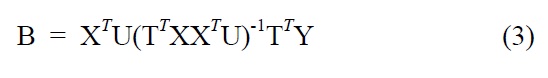
Finally, we can find the PLS calibration model as Y = XB +G, in which B represents PLS regression coefficients:

Similar to PLS algorithm, PCA can be used for solving regression problems, called principal component regression (PCR)[3].

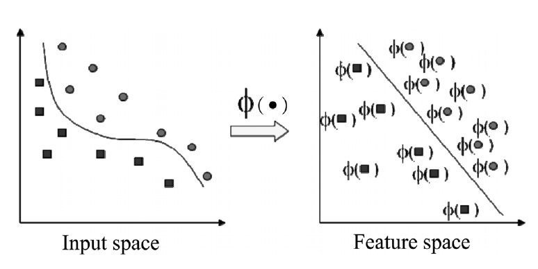
For nonlinear kernel methods to represent nonlinear patterns efficiently, the input data are mapped into a high dimensional feature space, in which a linear modeling of the data is possible as shown in Figure 1[7]. However, it is too difficult and troublesome to find the nonlinear mapping explicitly with computational problems due to the high dimensionality of the data. Thus, kernel functions have been used to overcome these problems[4]. The advantage of using kernel trick is that the learning in the feature space does not require explicit evaluation of the nonlinear mapping function.

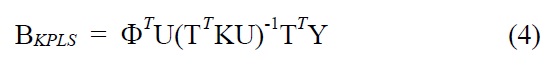
KPLS is the nonlinear kernel version of linear PLS. Similarly to KPCA, the introduction of kernel functions enables us to avoid both performing explicit nonlinear mappings and computing dot products in F. KPLS algorithm is directly derived from linear PLS algorithm with some modifications. As a result, regression coefficient matrix of KPLS has the form

The KPLS predictions from training (i.e., modeling building) data and test (i.e., independent validation) data can be obtained by

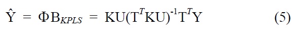
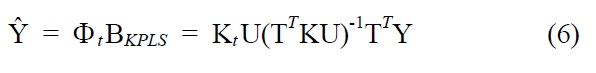
where Φ_t and Kt are the Φand the kernel matrix K for the test data points, respectively.

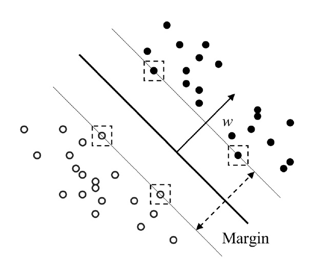
Similar to KPLS, the basic idea of support vector regression (SVR) is to map the data X into the feature space via a nonlinear mapping function, and then to do regression in this space. Mathematically, SVR is an extension of support vector machines (SVM) technique to regression problems. The details on SVM and SVR have been described elsewhere[5,9]. The optimal decision function is given by minimizing 1/2？w？² with inequality constraints y_i(wΦ(x_i) + b)-1 ≥ 0∀_i. By introducing ξ_i and Lagrangian, corresponding dual problem is givenby

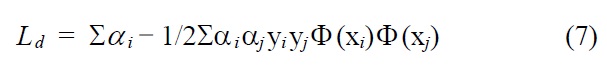
And the solution is calculated as w = Σ α_iy_iΦ (x_i), in which this is performed for support vectors with α_i > 0. Similar to other nonlinear techniques, the use of a kernel function K(x_i, x_j) allows the computation of dot products in a nonlinear feature space F without the use of nonlinear mappings. As shown in

Figure 2, an optimal separating hyperplane can be found which maximizes the margin.

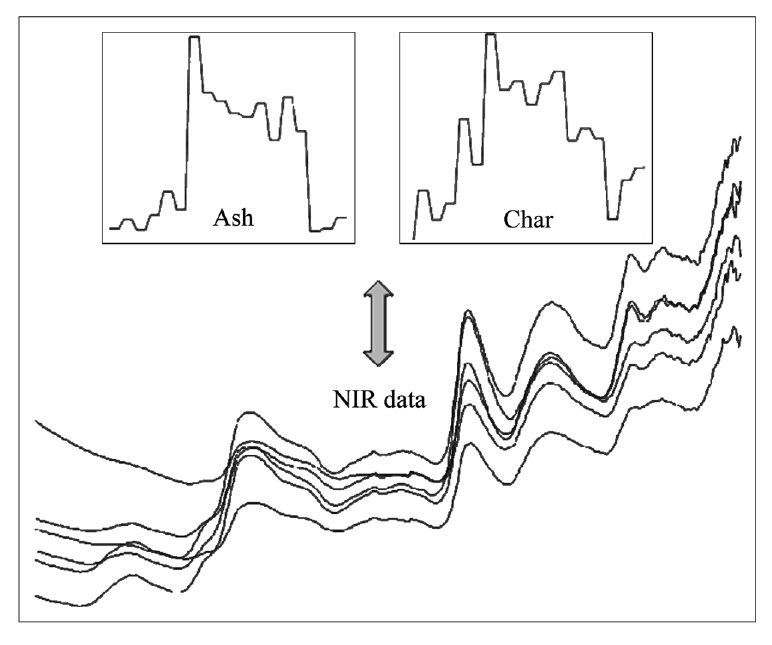
A total of six different biomass feedstocks were prepared for the prediction of ash and char contents based on NIR measurement data. For each of three wood species (redoak, hickory, and yellow poplar) and three others (switch grass, corn stover, and bagasse) three different samples were collected. NIR data for these biomass species were obtained with an advanced spectral devices (ASD) field spectrometer (wavelength range from 1,000 nm to 2,500 nm, Boulder, USA)[10]. The NIR data was reduced by averaging the 1 nm interval spectra to one with 4 nm intervals. Three spectra for each of 18 samples were obtained, and reflectance spectra were converted to absorbance spectra. NIR plots of some biomass samples are shown in Figure 3 including ash and char content. The measurement of ash content was performed via the recommended method of National Resources and Energy Laboratory (NREL) whilst char content was measured by thermal gravity analysis. The values for ash and char content range from the minimum 0.15 to the maximum 4.65 and from 11.65 to 21.79, respectively.

Prediction performance based on the biomass NIR data is presented. First, prior to performing NIR-based prediction of ash and char contents, some discrimination results are given here to show the advantage of using nonlinear techniques in this example. In general, the principal components or score values in reduced dimensions can be used to represent a big picture of the original data with different biomass groups or patterns. In terms of discrimination or classification, such a big picture

helps us to know the difference in NIR spectra data between various biomass species. Thus it can show an overall impression of how well the six different groups or clusters of the NIR data can be discriminated.

Along with linear PCA as described earlier, nonlinear kernel PCA was executed on the NIR spectra data to produce score plots. Similar to other nonlinear techniques, nonlinear kernel PCA needs to solve the eigenvalue problem

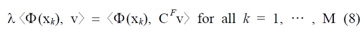
where C^F is the sample covariance matrix in the feature space. Then, there exists coefficients α_i, i = 1, … , M, such that v =

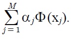
Finally combining these equations yields the following[4]:

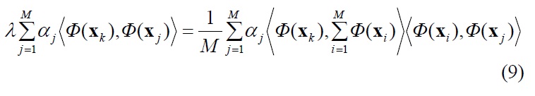
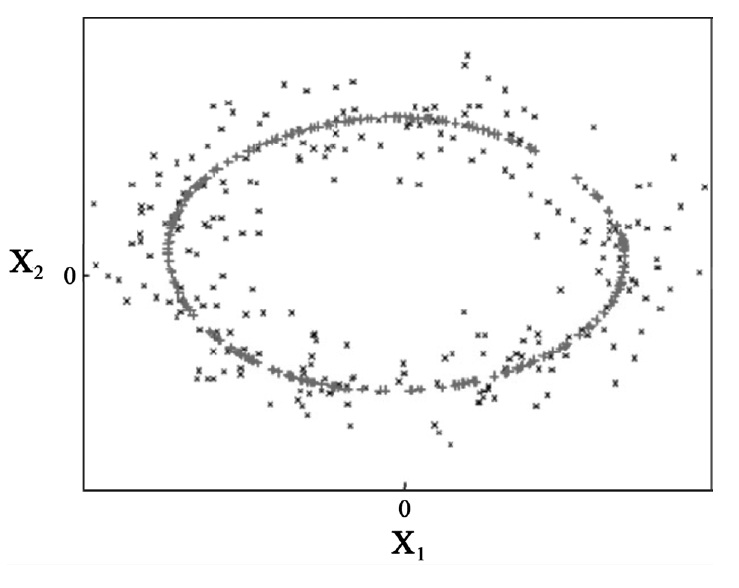
By applying a kernel function k(x_i, x_j) =〈Φ(x_i), Φ (x_j)〉, it is neither necessary to know Φ (x) nor we have to calculate dot products in F. As shown as a simple example in Figure 4, the application of KPCA to the original data with curvature facilitates better representation of nonlinear patterns of the data.

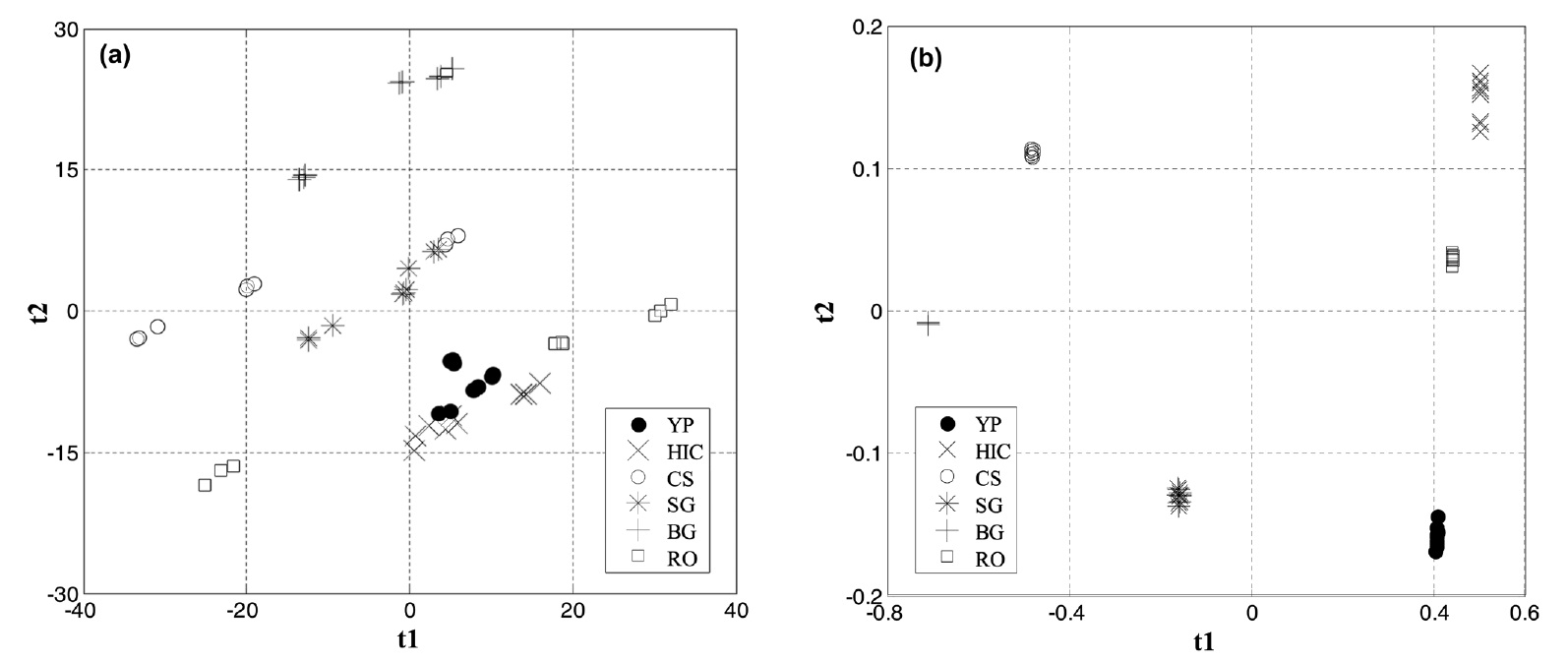
Figure 5 shows the score plots of the NIR data using linear PCA and nonlinear kernel PCA. The first two or three principal components usually can capture most of the variation of the data. Thus score plots based on selected principal components can facilitate visualization of different groups of data. However, linear techniques including linear PCA may have a limitation when they are applied to nonlinear data. Figures 5(a) and 5(b) show linear PCA and nonlinear kernel PCA score plots obtained from the NIR spectra, respectively. In these figures, YP represents yellow popular, HK hickory, CS corn stover, SG switchgrass, BG bagasse, and RO red oak. As shown in Figure 5(b), more clear discrimination of the NIR data between the six biomass species is obtained by nonlinear kernel PCA rather than linear PCA of Figure 5(a). It seems that visualization and discrimination is improved by taking into account the nonlinear characteristics of the NIR spectra data. For the nonlinear kernel PCA, a radial basis kernel function k(x, y) = exp(―？x― y？² / c was used to represent the NIR data. Actually, such a clear discrimination achieved by the nonlinear kernel PCA leads to less misclassification in classifying NIR samples between different biomass species. Here, the execution for the methods of this paper including KPCA was performed in an environment of MATLAB (MathWorks Inc., Natick, MA).

To evaluate the prediction performance for the biomass NIR data, several calibration models were built using a training data set and were tested on a test data set. Total four calibration models were constructed based on two linear techniques of PCR and PLS, along with two nonlinear techniques of KPLS, and SVR. In this work, leave-three-out procedure was executed on all 54 samples in order to increase the number of test data sets. While the NIR samples were not divided into simple two sets of training (for model-building) and test data (for validation), each of all samples was included in test data set. That is, three of the 54 samples was kept out of model development and predicted by the calibration model. Then, this task is repeated until every sample has been excluded only once. To compare the predictive abilities of the prediction models, root mean squared error for prediction (RMSEP) value was used and calculated based on the test data sets.

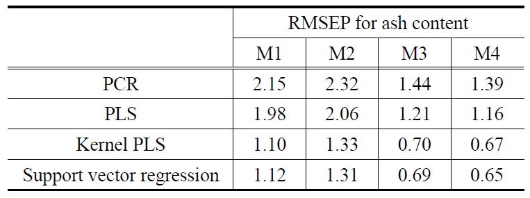
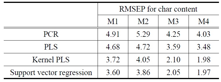
The prediction results for the biomass NIR data are summarized in Table 1 (for ash content) and Table 2 (for char content). In these tables, the influence of using different preprocessing methods on the prediction performance for ash and char contents is presented. In general, the optimum preprocessing method for NIR spectra depends on the type of data, and sample characteristics. Thus, there is no general rule for choosing the adequate pre-processing method. As shown in the tables, this work listed the effect of commonly used preprocessing methods such as no preprocessing (denoted as M1), multiplicative scatter correction followed by mean centering (denoted as M2), mean centering followed by orthogonal signal correction (denoted as M3), and second order derivative Savitsky-Golay followed by orthogonal signal correction (denoted as M4). These preprocessing methods for spectra data are a set of mathematical procedures on spectra.

For example, multiplicative scatter correction averages the spectra first, and each individual spectrum is regressed by partial least squares to the total average. The details about the preprocessing methods are out of scope of this work, and can beregerred elsewhere to other papers[2,11].

As shown in Table 1, RMSEP result for ash content using the two nonlinear calibration models show a significantly better prediction performance in that they produced less RMSEP values than linear models, irrespective of the preprocessing methods used. The linear calibration models using M4, for example, showed RMSEP values of 1.39 (for PCR) and 1.16 (for PLS) whilst the nonlinear models showed RMSEP values of 0.67 (for KPLS) and 0.65 (for SVR). Such observations can also be found from average RMSEP values calculated over the preprocessing methods (M1-M4). Average RMSEP values for each of the calibration models are obtained for the four preprocessing methods: 1.83 (PCR), 1.60 (PLS), 0.95 (KPLS), and 0.94 (SVR). The nonlinear SVR calibration model produced the lowest average RMSEP value of 0.94. It should be noted that, when compared to SVR, the KPLS model yielded similar good prediction performance with average RMSEP value of 0.95. Overall, the SVR prediction model with M4 showed the best prediction performance for ash content having the minimum RMSEP value (i.e., 0.65). The effect of using different preprocessing methods on prediction performance can be observed from Table 1. The M3 and M4 preprocessing methods produced similar RMSEP values. On the contrary, the use of M1 and M2 led to higher prediction errors for the four prediction models. This observation can be found by comparing average RMSEP values of each of the four preprocessing methods. Similar to the average RMSEP stated before, average RMSEP values calculated over the four prediction models were obtained from Table 1: 1.59 (M1), 1.76 (M2), 1.01 (M3), and 0.97 (M4).

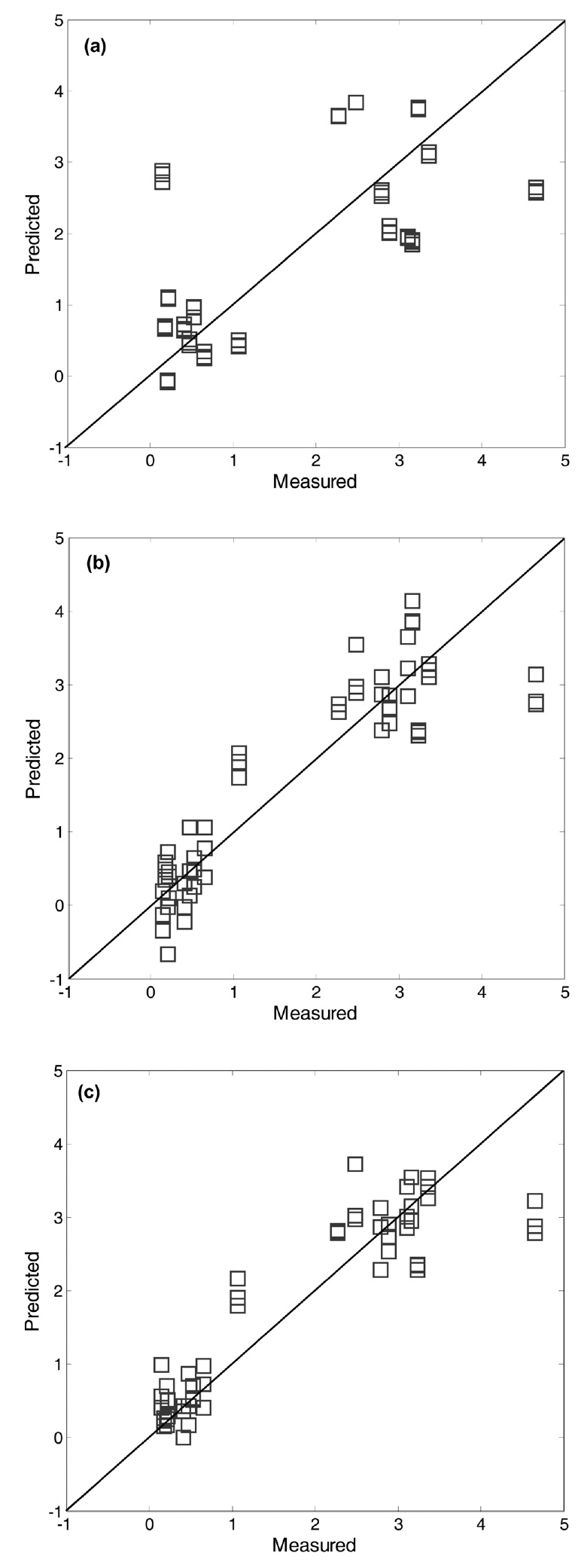
The predicted values of ash content for the test data were plotted against those observed in order to visualize the predictive performance of the prediction models. As shown in Figure 6, prediction results based on the threen models (i.e., PLS, KPLS, and SVR) are displayed for a comparison purpose, in which the preprocessing method of M4 was used. As expected from the RMSEP results, lown errors resulted in little dispersion around diagonal lines. Compared to the plot of the linear PLS model, the predicted vs. observed plots of the two nonlinearn models showed lessn errors. In such plots, the data points should fall on the diagonal. It means that then model predicts new test data perfectly. In this respect, it is observed that the two nonlinearn models have a better predictive ability than the linear PLS model. Actually, they produced reliable predicted values closer to the diagonal line than the linear PLS model.

Similar to the prediction results for ash content, those for char content were listed in Table 2. Overall prediction performance for char content showed that the two nonlinear prediction models outperformed the two linear models. Based on average RMSEP values calculated over the preprocessing methods, the SVR (KPLS) prediction model produced minimum average RMSEP value of 2.87 (2.96). However, average RMSEP values for the linear calibration models of PCR and PLS are 4.62 and 4.12, respectively. The best prediction results were obtained when using nonlinear prediction models with M4: 1.97 for SVR plus M4 and 1.98 for KPLS plus M4. In terms of the effect of the preprocessing methods used, in addition, average RMSEP values calculated over the four prediction models were obtained from Table 2: 4.23 (M1), 4.48 (M2), 3.00 (M3), and 2.87 (M4).

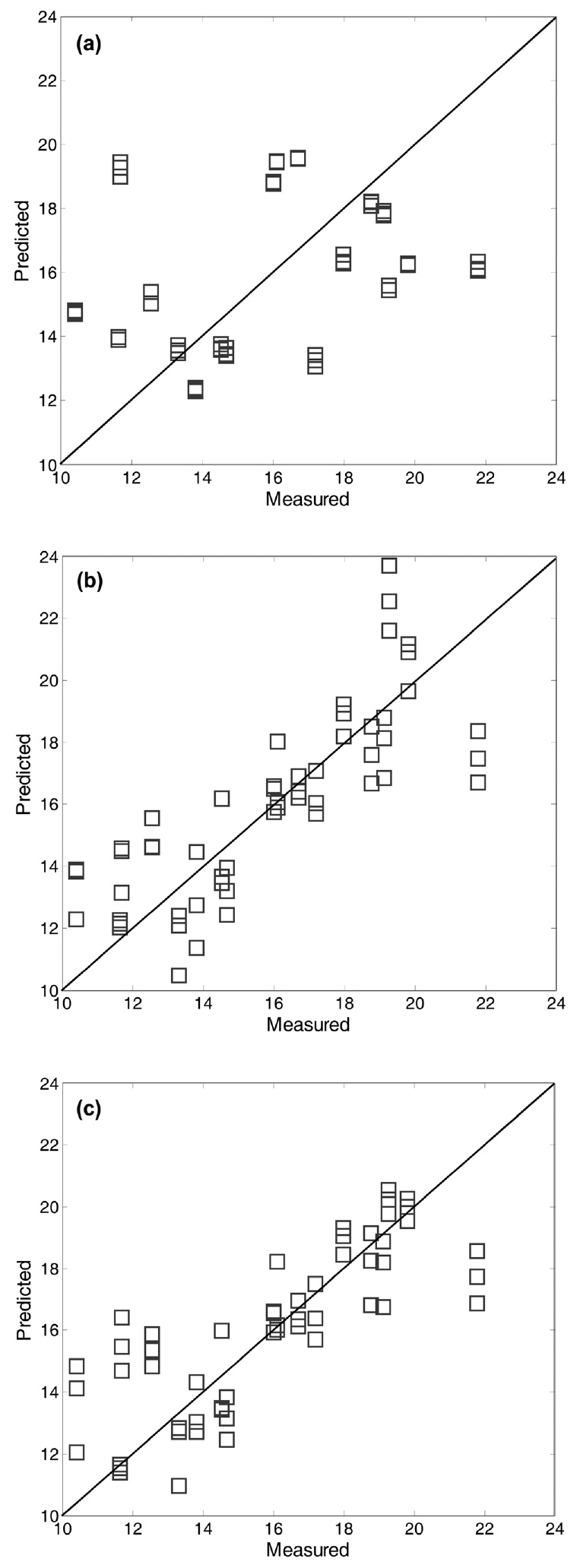
It is interesting to note that the predicted errors of M2 are higher than those of M1 (i.e., raw data used without preprocessing) : average RMSEP value 4.23 of M1 vs. 4.48 of M2. This trend is similar with the case of ash content. As listed in Table 1, average RMSEP value of M1 (1.59) is lower than M2 (1.76) for the ash prediction case. The use of preprocessing prior to building prediction models can be helpful in most of cases, but there may be a tradeoff between noise reduction and information loss [12]. On the other hand, it is worth noting that the RMSEP results illustrate the differences between linear techniques of the PCR and PLS. As shown in the two RMSEP tables, PLS yielded less prediction errors for ash and char contents than PCR. In fact, the PLS algorithm was known to be more efficient in extracting the information of NIR spectra data X that is strongly correlated with Y[2]. For a graphical comparison purpose, Figure 7 shows the plots of predicted vs. observed for biomass test data using different prediction models. As mentioned before, the nonlinear prediction models for char content have little dispersion around diagonal lines.

In this work, various prediction models coupled with different preprocessing methods were evaluated to predict biomass properties of ash and chart contents by NIR spectra data. The commonly used linear prediction techniques were applied and compared with nonlinear approaches. In addition, the score plots using linear and nonlinear PCA were constructed to facilitate visualization of different groups of biomass NIR data. As a result, visualization and discrimination between different biomass species was improved by adopting nonlinear PCA. In terms of prediction performance, the best prediction model was obtained when using nonlinear prediction models of SVR with a specific preprocessing method of M4. That prediction models with M4 produced the lowest prediction errors. In term of the effect of

using preprocessing methods for NIR data, preprocessing methods are a set of mathematical procedures which help to reduce noise of spectra data and increases signal from chemical information. Thus the use of preprocessing for spectra data including NIR usually results in a robust prediction model. However, predictive ability of a prediction model may deteriorate when there is an inappropriate selection of a preprocessing method. Thus, the optimal selection of preprocessing for a specific problem will require a trial and error process. The on-line prediction of biomass properties using NIR data with such a small error could be very beneficial for the production of bio-fuels. Also reliable knowledge of the quality of biomass will allow to run the production on tighter specifications and it will help reducing some of the raw material wastes.