Suicide is a major cause of death worldwide, with an annual global mortality rate of 16 per 100,000, and the problem is growing at a rate that has been increasing by 60% in the last 45 years [1]. Researchers have recently called for more qualitative research in the fields of suicidology and suicide prevention [2]. Computational methods can expedite such analyses by labeling related texts with relevant topics.
The work described in this paper was conducted in the context of track 2 of the 2011 Medical Natural Language Processing (NLP) Challenge on sentiment analysis in suicide notes [3]. This was a multi-label non-exclusive sentence classification task, where labels were applied to the notes left by people who died from suicide. This paper presents an evaluation of the utility of various types of features for supervised training of support vector machine (SVM) classifiers to assign labels representing topics including several types of emotion and indications of information and instructions. The information sources explored range from bag-of-words features and
We begin the remainder of the paper by providing some background on relevant work in Section II. We describe the data provided by the 2011 Medical NLP Challenge task organizers in Section III. Section IV details our approach, which involves training a collection of binary one-versus-all SVM sentence classifiers. Section V presents the performance of our approach, both under cross-validation of the development data and in final evaluation on held-out data. Section VI analyzes common types of errors, both in the gold-standard and the output produced by our system, while our conclusions and thoughts for future work are outlined in Section VII.
We are not aware of any previous work on the automatic labeling of suicide notes. However, given the emphasis on emotion labels, the most similar previous work is perhaps the emotion labeling subtask of the SemEval-2007 affective text shared task [4], which involved scoring newswire headlines according to the strength of six so-called basic emotions stipulated by Ekman [5] - ANGER, DISGUST, FEAR, JOY, SADNESS and SURPRISE. There were three participating systems in the SemEval- 2007 emotion labeling task. SWAT [6] employed an affective lexicon where the relevance of words to emotions was scored in an average emotion score for every headline in which they appear. UA [7] also used a lexicon, which was instead compiled by calculating the point-wise mutual information with headline words and an emotion using counts obtained through information retrieval queries. UPAR7 [8] employed heuristics over dependency graphs in conjunction with lexical resources such as WordNet-Affect [9]. In subsequent work, the task organizers investigated the application of latent semantic analysis (LSA) and a Naive Bayes (NB) classifier that was trained using author-labelled blog posts [10]. As can perhaps be expected given the different approaches of the various systems, each performed best for different emotions. This highlights the need for emotion-labeling systems to draw from a variety of analyses and resources.
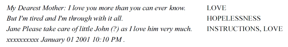
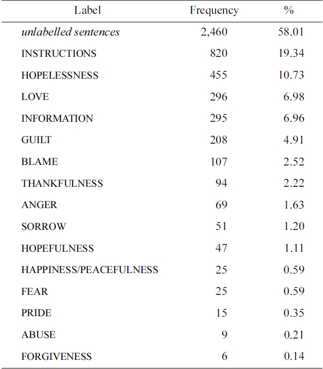
The task organizers provided developmental data consisting of 600 suicide notes, comprising 4,241 (pre-segmented) sentences. Note that a “sentence” here is defined by the data, and can range from a single word or phrase to multiple sentences (in the case of segmentation errors). Each sentence is annotated with 0 to 15 labels (listed with their distribution in Table 1). For held-out evaluation, the organizers provided an additional set of 300 unlabelled notes, comprising 1,883 sentences. The task organizers report an inter-annotator agreement rate of 54.6% over all sentences. Fig. 1 provides excerpts from a note in the training data, with assigned labels.
Our approach to the task of labeling suicide notes
[Table 1.] The distribution of labels in the training data

The distribution of labels in the training data
involves learning a collection of binary
The classifiers are based on the framework of SVM [12]. SVMs have been found to be very effective for text classification and tend to outperform other approaches such as NB [13]. For each label, we train a linear sentence classifier using the SVM
We explored a range of different feature types for our emotion classifiers. The most basic features we employ are obtained by reducing inflected and derived words to their stem or base form, e.g.,
Another feature type records
Lexicalized Part-of-Speech features are formed of word stems concatenated with their part-of-speech (PoS). PoS tags are assigned using TreeTagger [17], which is based on the Penn Treebank tagset.
Features based on syntactic dependency analysis provide us with a method for abstracting over syntactic patterns in the data set. The data is parsed with Maltparser, a language-independent system for data-driven dependency parsing [18]. We train the parser on a PoS-tagged version of the Wall Street Journal sections 2-21 of the Penn Treebank, using the parser and learner settings optimized for the Maltparser in the CoNLL-2007 Shared Task. The data was converted to dependencies using the Pennconverter software [19].
The parser was chosen partly due to its robustness to noise in the input data; it will not break down when confronted with incomplete sentences or misspelled words, but will always provide some output. While the amount of noise in the data will clearly affect the quality of the parses, we found that, in the context of this task, having at least some output is preferable to no output at all.
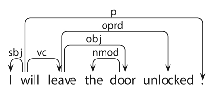
Consider the dependency representation provided for the example sentence in Fig. 2. The features we extract from the parsed data aim to generalize over the main predication of the sentence, and hence center on the root of the dependency graph (usually the finite verb) and its dependents. In the given example, the root is an auxiliary, and we traverse the chain of verbal dependents to locate the lexical main verb,
Sentence dependency patterns: lexical features (wordform, lemma, PoS) of the root of the dependency graph, e.g., (leave, leave, VV), and patterns of dependents from the (derived) root, expressed by their dependency label, e.g., (VC-OBJ-OPRD), partof- speech (VV-NN-VVD) or lemma (leave-doorunlock)
Dependency triples: labelled relations between each head and dependent: will-SBJ-I, will-VCleave, leave-OPRD-unlocked, etc.
We also include a class-based feature type recording the semantic relationships defined by WordNet synonym sets (synsets) [20]. These features are generated by mapping words and their PoS to the first synset identifier (WordNet synsets are sorted by frequency). For example, the adjectives
WordNet-Affect [9] is an extension of WordNet with affective knowledge pertaining to information such as emotions, cognitive states, etc. We utilize this information by activating features representing emotion classes when member words are observed in sentences. For example, instances of the words
In preliminary experiments, we investigated the difference in performance when representing feature frequency versus presence, as previous experiments in sentiment classification [21] indicated that unigram presence (i.e., a boolean value of 0 or 1) is more informative than their frequencies. For the suicide note analysis, however, we found that features encoding frequency rather than presence always performed better in our end-to-end experiments.
The final type of feature that we will describe represents the degree to which each stem in a sentence is associated with each label, as estimated from the training data. While there is a range of standardly used lexical association measures that could potentially be used for this purpose (such as point-wise mutual information, the Dice coefficient, etc.), the particular measure we will be using here is the
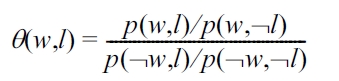
If the probability of having the label
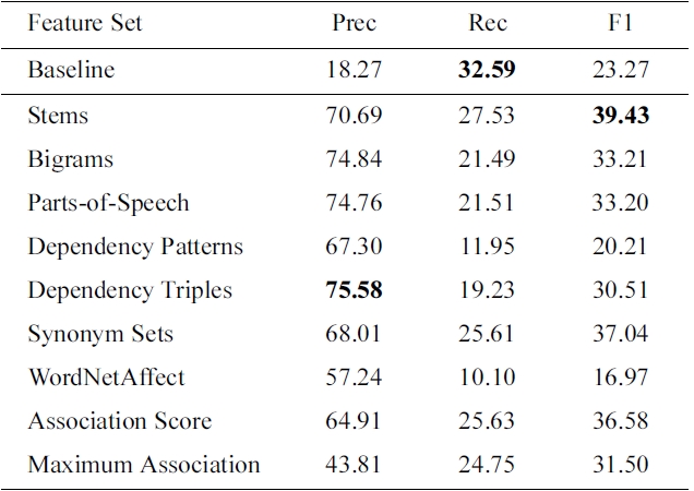
Developmental results of various feature types. The baseline corresponds to labeling all items as instructions, the majority class
boolean features indicating which label had the maximum association score.
From the frequencies listed in Table 1, it is clear that the label distributions are rather different. Moreover, for each individual classifier, it is also clear that the class balance will be very skewed, with the negative examples (often vastly) outnumbering the positives. At the same time, it is the retrieval of the positive minority class that is our primary interest. A well-known approach for improving classifier performance in the face of such skewed class distributions is to incorporate the notion of
As specified by the shared task organizers, overall system performance is evaluated using micro-averaged F1. In addition, we also compute precision, recall and F1 for each label individually. We report two rounds of evaluation. The first was conducted solely on the development data using ten-fold cross-validation (partitioning on the note-level). The second corresponds to the system submission for the shared task, i.e., training classifiers on the full development data and predicting labels for the notes in the held-out set.
Table 2 lists the performance of each feature type in isolation (using the same feature configuration for each binary classifier and the default symmetric cost-balance). We also include the score for a simple baseline method that naively assigns the majority label (INSTRUCTIONS) to all sentences. We note that stems are the most informative feature type in isolation and perform best overall (F1 = 39.43). Dependency Triples are most effective in terms of precision, and all feature types have less recall than the majority baseline.
In further experiments that examined the effect of using several feature types in combination, we found that combining stems, bigrams, parts-of-speech and dependency analyses achieved the best performance overall (F1 = 41.82). However, these experiments also made it clear that different combinations of features were effective for different labels. Moreover, as our one-versus-all set-up means training distinct classifiers for each label, we are not limited to using one set of features for all labels. We therefore experimented with a grid search across different permutations of feature configurations, as further described below.
We also tuned the cost-balance parameter described in Section IV above. The reason for introducing the costbalance parameter in our setup is to alleviate the imbalance between positive and negative examples. For some labels, this imbalance is so extreme that our initial system was unable to identify any positive predictions at all, neither true nor false. An example of such a label is forgiveness, which has only six annotated examples among the 4,241 sentences in the training data. Naturally, any supervised learning strategy will have problems making reliable generalizations on the basis of so little evidence. However, even for the more frequently occurring labels, the ratio of positive to negative examples is still quite skewed.
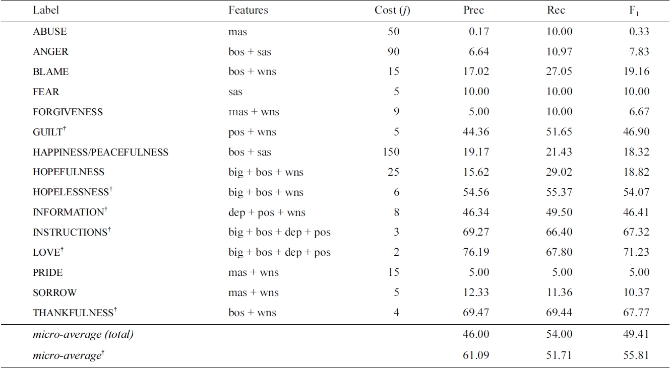
As we found that the optimal feature configuration was dependent on the value of the cost-balance parameter (and vice-versa), these parameters were optimized in parallel for each classifier. The results of this search are listed in Table 3, with the best feature combinations and cost-balance for each label. We note that the optimal configuration of features varies from label to label, but that stems and synonym sets are often in the optimal setup, while dependency triples and features from WordNetAffect do not occur in any configuration.
As discussed above, the unsymmetric cost factor essen-

Labels in the suicide notes task with feature sets and cost-balance (j) optimized with respect to the local label F1
tially governs the balance between precision and recall. For many classes, increasing the cost of errors on positive examples during training allowed us to achieve a pronounced increase in recall, though often at a corresponding loss in precision. Although this could often lead to greatly increased F1 at the level of individual labels, the overall micro F1 was compromised due to the low precision of the classifiers for infrequent labels in particular. Therefore, our final system only attempts to classify the six labels that can be predicted with the most reliability - GUILT, HOPELESSNESS, INFORMATION, INSTRUCTIONS, LOVE and THANKFULNESS - and makes no attempt on the remaining labels.
Testing by ten-fold cross-validation of the development data, this has the effect of an increased overall system performance in terms of the micro-average scores (compare
Table 4 describes the performance on the held-out evaluation data set when training classifiers on the entire development data set, with details on each label attempted by our setup. As described above, we only apply classifiers for six of the labels in the data set (due to the low precision observed in the development results for the remaining nine labels). We find that the held-out results are quite consistent with those predicted by cross-validation on the development data. The final micro-averaged F1 is 54.36, a drop of only 1.45 compared to the development result (see Section VII for a comparison of our system and its
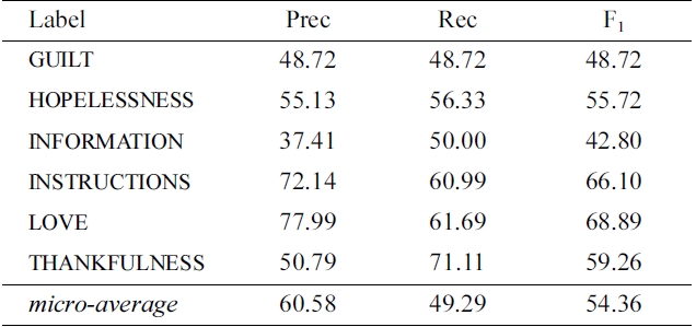
Performance of our optimized classifiers trained using the development data and tested on the held-out evaluation data
results to those of other participants in the shared task).
This section offers some analysis and reflections with respect to the prediction errors made by our classifiers. Given the multi-class nature of the task, much of the discussion will center on cases where the system confuses two or more labels. Note that all example sentences given in this section are taken from the shared task evaluation data and are reproduced verbatim.
In order to uncover instances of systematic errors, we compiled contingency tables showing discrepancies between the decisions of the classifiers and the labels in the gold standard. Firstly, we note that BLAME and FORGIVENESS are often confused by our approach, and are closely related semantically. We consider these classes to be polar in nature; while both imply misconduct by some party, they elicit opposite reactions from the offended entity. Their similarity means that their instances often share features and are thus confused by our system.
We also note that the classes of GUILT and SORROW are hard to discern, not only for our system but also for the human annotators. For instance, Example 1 is annotated as SORROW, while Example 2 is annotated as GUILT. This makes features such as the stem of
Example 1. Am sorry but I can’t stand it ...
Example 2. I am truly sorry to leave ...
Example 3. ... sorry for all the trouble .
It is worth noting here that some of the apparent inconsistencies observed in the gold annotations are likely due to the way the annotation process was conducted. While three annotators separately assigned sentence-level labels, the final gold standard was created on the basis of majority vote between the annotators. This means that, unless two or more annotators agree on a label for a given sentence, the sentence is left unlabelled (with respect to the label in question).
Some of the labels in the data tend to co-occur. For instance, Example 1 above is actually annotated with both SORROW and HOPELESSNESS. However, these intuitively apply to two different sub-sentential units:
Note that the problem discussed above is also compounded due to errors in the sentence segmentation. For instance, Example 4 is provided as a single sentence in the training data, with the labels THANKFULNESS and HOPELESSNESS. However, as the labels actually apply to different sentences, this will introduce additional noise in the learning process.
Example 4. You have been good to me. I just cannot take it anymore.
Some of the errors made by the learner seem to indicate that having features that are sensitive to a larger context might also be useful, such as taking the preceding sentences and/or previous predictions into account. Consider the following examples from the same note, where both sentences are annotated as INSTRUCTIONS:
Example 5. In case of accident notify Jane.
Example 6. J. Johnson 3333 Burnet Avenue.
While Example 6 is simply an address, it is annotated as INSTRUCTIONS. Of course, predicting the correct label for this sentence in isolation from the preceding context will be near impossible. Other cases would seem to require information that is very different from that captured by our current features, such as pragmatic knowledge, before we could hope to get them right. For example, in several cases, the system will label something as INFORMATION when the correct label is INSTRUCTIONS. This is often because a sentence has communicated information which pragmatically implied an instruction. For example, we presume that Example 7 is annotated as INSTRUCTIONS because it is taken to imply an instruction to collect the clothes.
Example 7. Some of my clothes are at 3333 Burnet Ave. Cincinnati - just off of Olympic .
This paper has provided experimental results for a variety of feature types for use when learning to identify various fine-grained emotions, as well as information and instructions, in suicide notes. These feature types range from simple bags-of-words to syntactic dependency analyses and information from manually-compiled lexicalsemantic resources. We explored these features using an array of binary SVM classifiers.
A challenging property of this task is the fact the classifiers are subject to extreme imbalances between positive and negative examples in the training data; the infrequency of positive examples can make the learning task intractable for supervised approaches. In this paper, we have shown how a cost-sensitive learning approach that separately optimizes the cost-balance parameter for each of the topic labels, can be successfully applied for addressing problems with such skewed distributions of training examples. For the less-frequent labels, however, the optimal F1 tended to arise from gains in recall at the great expense of precision. Thus, we found that discarding poorly-performing classifiers resulted in improvements overall. While arguably an ad hoc solution, this is motivated by the shared task evaluation scheme of maximizing micro-averaged F1.
Of the twenty-five submissions to the shared task, our system was placed fifth (with a micro-averaged F1 of 54.36); the highest-performer achieved an F1 of 61.39, while the lowest scored 29.67. The mean result was 48.75 (
An analysis of the errors made by our system has suggested possible instances of inter-annotator confusion, and has provided some indications for directions for future work. These include re-annotating data at the subsentential level, and drawing in the context and predictions of the rest of the note when labeling sentences. We also note that text in this domain tends to contain many typographical errors, and thus models might benefit from features generated using automatic spelling correction.
In other future work, we will conduct a search of the parameter space to find optimal parameters for each label with respect to the overall F1 (rather than the label-local F1 we used in the current work). Finally, we will look to boost performance for labels with few examples by drawing information from large amounts of unlabelled text. For instance, inferring the semantic similarity of words from their distributional similarity has been effective for other emotion-labeling tasks [28].