Object tracking is an important task for many applications, such as for robot navigation, surveillance, automotive safety, and video content indexing. Based on trajectories obtained through tracking, some advanced behaviour analysis can be applied. For instance, a pedestrian’s trajectory can be analysed to warn a driver if the trajectories of the vehicle and of the pedestrian are potentially intersecting.

For multiple object tracking, tracking-by-detection methods are the most popular algorithms. A detector is used in each image frame to obtain candidate objects. Then, with a data-association procedure, all the candidates are matched to the existing trajectories as known up to the previous frame. Any unmatched candidate starts a new trajectory. Since there is no perfect detector that detects all objects without any false positives and false negatives, sometimes objects are missed (i.e., they appear in the image but are not detected), or background windows are incorrectly detected as being objects. Such false-positive or false-negative detections increase the difficulty of tracking.

Occlusion by other objects or the background is one of the main reasons for detection to fail and it also increases the difficulty of tracking (e.g., identity switch). Some algorithms [1,2] propose tracking objects in the 2D image plane. The occlusion problem is handled either using part detectors and tracking detected body parts, or adopting instance-specific classifiers to improve performance of data assignment. However, tracking in the 2D image plane increases the ambiguity of data association. A tall person nearby, and a small person far away, for example, may appear very close to each other in the image, and, possibly, in some frames the tall person occludes the small person. But they are actually several meters away from each other. Thus, often, and also in this paper, stereo information is adopted to improve the tracking performance [3-5], and multiple pedestrians are tracked in 3D coordinates.

Tracking objects with irregular movements in 3D space is a challenging task due to the totally unknown speed and direction. In this paper, the application of an unscented Kalman filter (UKF), which can also handle nonlinear?in fact, fully irregular trajectories in 3D space, is demonstrated. For the original paper on UKF see [6]. Similar work is proposed in [5]. However, instead of modelling the motion of the vehicle and the pedestrians separately, we straightforwardly model the relative motion between them, and no ground plane is assumed, so that objects moving with 6 degrees of freedom can be tracked properly. Different types of models are tested and compared in both simulation and real sequences.

Multiple object tracking has attracts a great deal of attention recently in computer vision research. Today, an update of the review [7] from 2006 should also include work such as in [2-4,8-13].

Kalman filters (KF) have been extensively adopted to deal with tracking tasks. A KF is a recursive Bayesian filter, firstly, using motion information to predict the possible position, followed by fusing the observation (detection) and predicted position. A linear KF is used for tracking (e.g., [7]) when movement is such that linear models may be used for approximation. Obviously, a linear model is not suitable for most cases. The extended Kalman filter (EKF) was designed [14] for handling a nonlinear model by linearizing functions using the Taylor expansion extensively. For example, an EKF has been used for simultaneous localization and mapping [15], and for pedestrian tracking [16]. A particle filter was used to handle the task in [17]. Performance similar to an EKF is reported in [3].

The UKF can handle a nonlinear model by using the unscented transform to estimate the first and second order moments of sigma points, which represent the distribution of a predicted state and predicted observations, and it appears that the UKF does this better than the EKF [18]. Thus, in this paper, a UKF is used for tracking multiple, irregularly moving objects in 3D space, which is a highly nonlinear problem.

The unscented transform (UT) is the core component that enables the UKF able to be able to handle nonlinear models. Let L be the dimensionality of the system state x_t-1|t-1 at time t-1. If the system noise (process noise Q and measurement noises R) is not additive noise, the state is augmented before UT. In our case, random acceleration is introduced as process noise; thus, the state augmented with a process noise vector, is denoted by

and called vector for short. The dimension of the augmented vector depends on the process model, which is illustrated in Section IV. Let x_t|t-1 denote the predicted state at time t when passing x_t-1|t-1 through process function f. Let y_{t |t -1} be the predicted observation at time t when passing x_{t |t -1} through observation function h.

The UT works by sampling 2L+1 sigma vectors X_i^(a) in the augmented state space (following [6]), forming a matrix χ ^(a) . The covariance matrix in augmented state space is denoted by P^(a). Let

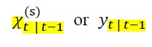
be the state covariance matrix (i.e., describing dependencies between components of a state χ ). Formally,

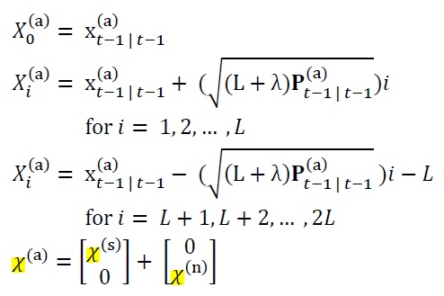
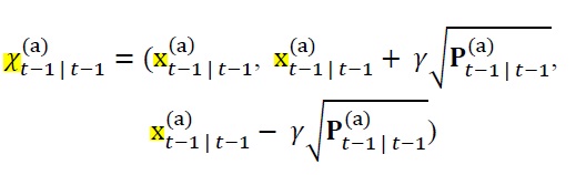
where λ is a positive real, used as a scaling parameter. These sigma vectors can be passed through a nonlinear function (e.g., f or h) one by one, thus defining trans-formed (i.e., new) sigma vectors such as

Means x_t|t-1 or y_t|t-1 and covariance matrices

are obtained as follows; take h for example:

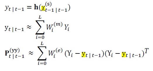
with constant weights W_i^(.). Details are given in [6].

The UKF is illustrated as follows. At first we initialize the state x=x₀ and state covariances P^(xx) = P₀^(xx). For the augmented vectors, let

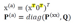
where Q denotes the process-noise covariance matrix. Details about Q are given in Section IV. For t ？ (1, … , ∞), we calculate sigma vectors as follows:

The process update is as follows:

We update the sigma vectors using

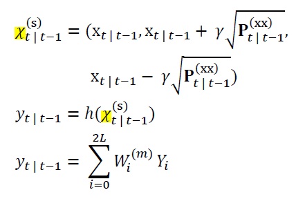
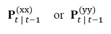
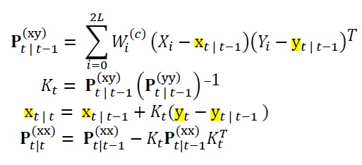
and update the measurement covariance matrix as follows:

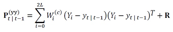
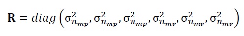
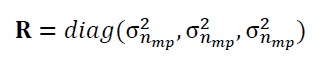
where R is the assumed measurement noise covariance, depending on the observation model selected. Details are given in Section IV.

Altogether, the UKF is defined by

Following tracking-by-detection methods, which are popular for solving multiple-object tracking tasks, a detector is applied in each frame to generate object candidates which are outputs of the detector. One UKF is adopted for tracking one object separately; thus a group of detected pedestrians defines a family of UKFs to be processed simultaneously. Each UKF tracks one detected object. The predicted state of a UKF is used for data association; when an observation (of the tracked object) is available in the current frame then we update the predicted state by using the corresponding UKF.

Detection-by-tracking methods rely on evaluating rectangular regions of interest, and we call them object boxes if positively identified as containing an object of interest. For pedestrian tracking, we adopt the popular histogram of oriented gradients (HOG) feature method and a support vector machine (SVM) classifier, originally introduced in [19]. HOG features describe the human profile by an oriented gradient histogram. An SVM classifier is able to handle high-dimensional and nonlinear features (such as HOG features). It projects sample features into a high

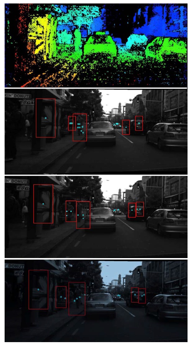
dimensional space, and then finds a hyperplane to separate two classes. Instead of using a sliding window, regions of interest (i.e., inputs to the classifier) are selected by analysing calculated stereo information (depth and disparity maps), as proposed in [20].

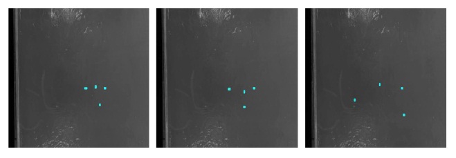
Fig. 1 shows several detection results in pedestrian sequence, dots (cyan) denote the boxes’ centre that are recognized as pedestrians, and the red rectangles denote the final detection results. As can be seen in the results, the object boxes may contain background, shift from the object, or miss the pedestrians.

For the detection of Drosophila larvae (an example of 2D movement), thresholds and connected components are adopted to obtain one object box for each larva. Several larva detection results are shown in Fig. 2. As the scene is certain, the detection results are more reliable when compared to the pedestrian sequence. However, no depth information is available here.

As there is an unknown number of objects in a scene, the state-dimensionality would expand significantly if we would have decided to track all pedestrians in one UKF; in this case, the speed of tracking reduces dramatically when the scene is crowded with many detected objects. Thus, we decided on one UKF for each detected object for tracking.

Choosing a proper model is important. In this subsection we offer three models for possible selection: 3DVT means that 3D position (world coordinates) with velocity is observed, 3DT means that 3D position without velocity is observed, and 2DT means that 2D position (image coordinates) without velocity is observed. These models are compared in Section V.

1) The Two 3D Models

In the 3DVT model, the object is tracked in 3D world coordinates. Its 3D position (x, y, z) is the first part of the state. We also include the velocity (v_x, v_y, v_z). Thus, a state x=(x, y, z, v_x, v_y, v_z)^T is 6-dimensional.

a) Process model: We assume constant velocity between adjacent frames, with Gaussian distributed noise acceleration na ？ N (0, Σna). The diagonal elements in Σna are set to be equal and denoted by

Thus,

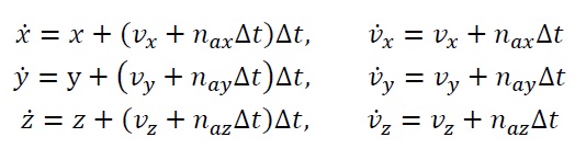
whereΔt is thetime interval between subsequent frames.

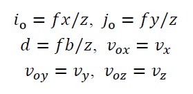
b) Observation model: An observation consists of the position (i0, j0) (say, the centroid of the detected object box in the left camera), disparity d of the detected object, and velocity (vox, voy, voz) in 3D coordinates. The usual pinhole camera projection model is used 4to map 3D points onto the image plane,

where f denotes focal length, and b denotes the length of the baseline between two rectified stereo cameras. In this case,

For the disparity d we select the mode in the disparity map in a fixed (e.g., 20 × 20) neighbourhood around the centroid (i₀, j₀ ) of the detected object box. 3D scene flow (v_ox, v_oy, v_oz) can be obtained by combining optic flow and stereo information [21].

As it is difficult to obtain high-quality scene flow as required for 3DVT, 3DT simplifies the 3DVT model by excluding the scene flow from the observation, and has the same process model as 3DVT. In this case,

2) The 2D Model

If only monocular recording is available, the object is tracked in the 2D image plane only. The state x=(i,j,v_i,v_j)^T consists of position (i, j) and velocity (v_i, v_j).

a) Process model: The process model is the same as for the 3D models. We assume a constant velocity between subsequent frames with a Gaussian noise distribution for acceleration n_a:

b) Observation model: An observation consists of the central position (i₀, j₀) of an object box only, i₀ = i and j₀ = j, resulting in R = diag(σ²_nmp,σ²_nmp) for this case.

C. Data Association

As each object is tracked independently, data association by matching candidates to existing trajectories becomes important. If no match is found then we decide to initialize a new tracker.

Since object movements are continuous, the estimated velocity in the UKF can be used as a cue to localize the search area in order to find the match object. For each trajectory, the possible location (i.e., (x_p, y_p, z_p) for 3D, and (i_p, j_p) for 2D) of the object in the current frame is predicted by a process model used in the EKF. This location is used as a reference for searching potentially matching candidates in the current frame. Currently we simply match candidates based on the shortest Euclidean distance and a given threshold T.

One candidate might be matched with several trajectories if the Euclidean distance is below T. Trajectories compete for the candidates, and in the end, the closest one wins. If a candidate is not matched to any trajectory, a new tracker is initialized. If a trajectory does not win any of the candidates, the tracker is propagated with the given prediction, and the new state is the predicted state, without being updated by an observation (because it is not available).

No object appearance description is used here for assigning an object to a trajectory. In general, the inclusion of appearance representation (e.g., a colour histogram, or an instance-specific shape model) improves the performance. However, this is out of the scope of this paper, where we are focusing on the combination of different data association methods.

In this section, first, our three models (3DVT, 3DT, and 2DT) are tested in a simulated environment with different parameter sets. Second, our multiple-object tracking method is tested on real video sequences where (3D example) pedestrians are walking in inner-city scenes, or (2D example) larvae are moving on a flat culture dish.

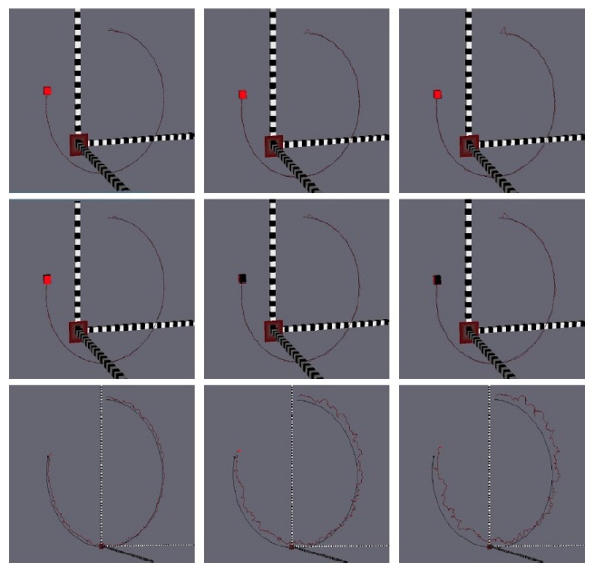
The three models defined in Section IV are tested in a simulation environment in OpenGL (SGI, Fremont, CA, USa). A cub is moving on a circular path around a 3D point with constant speed, as shown in Figs. 3 and 4. Acceleration noise n_a with different covariance (e.g., σ²_na = 0.0001, 0.01, 1), and measurement noise n_m with different covariance (e.g., σ²_nmp = 10, 50, 100, σ²_nmv = 50, 100, 150), are used to test and compare the three models’ performance. The simulation environment is different for 2D and 3D models, where for 2D, positions are integral pixel coordinates in the image plane, but for 3D, position coordinates are reals. The radius of the circle in the 3D models is 10, while in the 2D model it is 50. In both environments, measurements are degraded by noise before being sent to the UKF.

Fig. 3 demonstrates the effect of σ²_na, having fixed σ²_nmp and σ²_nmv. Experiments show that larger σ²_na values result in more unstable trajectories. A large σ²_na means that the process model produces a predicted state that is fluctuating with large magnitudes. Results show that σ²_na = 0.0001 is a reasonable choice for 3D models. For the 2D model, a smaller σ²_na yields smooth estimation, but the shifts are significant.

A larger σ²_na value produces estimations that are closer to the true positions, but fluctuations are significant, for an experiment with σ²_na =1 for the 2D case. In general, 3DT and 3DVT converge better than 2DT, while 3DT and 3DVT show a similar performance. 3D models use stereo information rather than just a single image as for the 2D model, which also proves that stereo information can help to improve the tracking performance. As the measured 3D position is noisy, the measure of velocity is even noisier; this appears to be the main reason for the observation that the inclusion of velocity cannot improve the performance.

Fig. 4 shows results for our models for different covariance values σ²_nmp and σ²_nmv of measurement noise. Significantly increasing measurement noise (i.e., higher uncertainty of observations) reduces the performance only slightly. This demonstrates that, to some degree, the UKF is a robust tracker, which is not vulnerable to detection uncertainties. As before, 3DT and 3DVT converge better than 2DT, while 3DT and 3DVT show a similar performance.

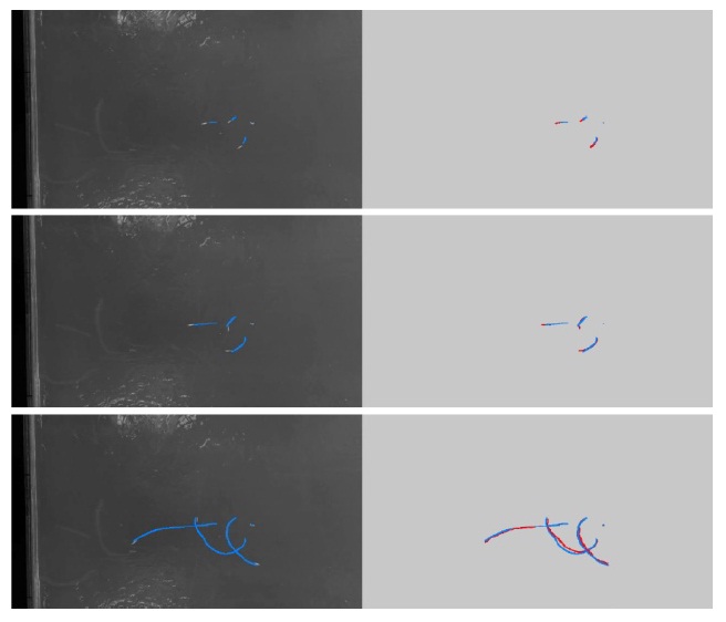
In this section we report on the performance of UKFsupported tracking for multiple larvae using the 2DT model, and for multiple pedestrians in traffic scenes using the 3DT model. The larvae and pedestrian sequences are recorded at 30 and 15 frames per second, respectively.

Results for larvae tracking are shown in Fig. 5. As the velocity in the model is initialized by (0,0), the UKFestimation is “ slower” than the real speed of the larvae in the first 30 frames. The speed of convergence can be improved by increasing σ²_na, but it should be noted that the larger the σ²_na value is, the larger the magnitude of fluctuation. The estimated trajectories follow the moving larvae effectively, mainly because all of the larvae are properly detected in all of the frames. However, such a complete detection cannot be expected for pedestrian sequences. Next, we test the UKF for such “ noisy” detection results as pedestrian sequences.

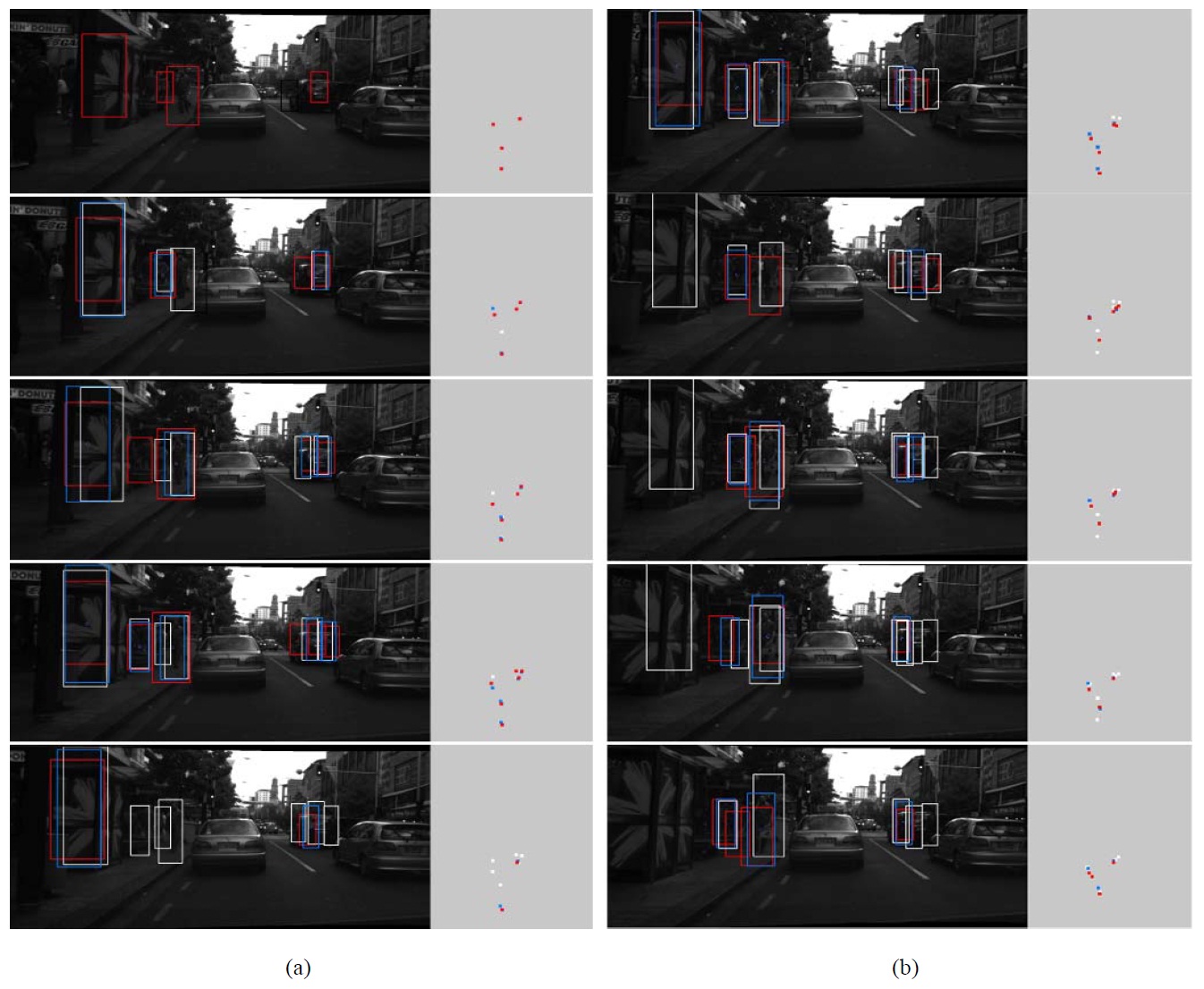
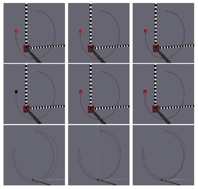
The results for pedestrian tracking are shown in Fig. 6. Objects are missing or shifting from time to time due to the clustered background (e.g., the car in the traffic scene detected as a pedestrian), illumination variations leaving some pedestrians undetected, or internal variations between objects (i.e., unstable detections). Our experiments verified that UKF predictions are able to follow irregularly moving pedestrians when detection fails for a few frames, and can even correct unstable detections.

The second frame in Fig. 6 shows that the undetected pedestrian is predicted correctly in the white object box and is successfully matched to a detected position in the third frame. The last frame in Fig. 6 demonstrates that displaced detections are corrected by the UKF. Using only the defined distance rule for data assignment, this appears to be insufficient, especially for the given detection results. A small threshold may lead to a mismatch (i.e., the detection fails to satisfy the rule), and a large threshold may lead to an identity switch (i.e., a pedestrian is matched to another pedestrian).

Assigning one UKF to each detected (moving) object simplifies the design and implementation of UKF prediction of 2D or 3D motion. Experiments demonstrate the robustness of the chosen approach. This tracker only generates shortterm tracks when detection is not reliable; long-term tracking should be possible by also introducing dynamic programming.

For evaluating the performance in real-world (either 2D or 3D) applications, more extensive tests need to be undertaken, especially for the design and evaluation of quantitative performance measures. For example, the measures discussed in [22] for evaluating visual odometry techniques might also be of relevance for the tracking case.