검색 전체 메뉴
PDF
맨 위로
OA 학술지
Simple Spectral Calibration Method and Its Application Using an Index Array for Swept Source Optical Coherence Tomography
  • 비영리 CC BY-NC
  • 비영리 CC BY-NC
ABSTRACT
Simple Spectral Calibration Method and Its Application Using an Index Array for Swept Source Optical Coherence Tomography
KEYWORD
OCT , K-linearization , Spectral calibration , SS-OCT , Signal processing
  • I. INTRODUCTION

    Optical coherence tomography (OCT) is a non-invasive and non-contact technology that can show a biological imaging section with a high resolution of 1~15 μm [1-2]. OCT is classified into time domain (TD) and frequency domain (FD)-OCT according to the structure of the reference arm optics. And the FD-OCT is classified into swept source (SS) and spectral domain (SD)-OCT according to the output characteristics of the light source and the structure of light receiving components [3]. FD-OCT has inevitable nonlinearity in the k-triggering because of the hardware characteri-stics from the light source, the spectrometer, and the optical components [4].

    In the FD-OCT system using the inverse Fourier transform relationship of the interference pattern, the nonlinearity to the k-domain diminishes the depth resolution. Several attempts have been made to compensate such nonlinearity [5-12]. There are some compensation methods for various OCT systems. One is a compensation method that inserts the interferometer into the SS-OCT system, receives the linearized interference pattern to the k-triggering and uses the pattern as a trigger signal [5]. Another method is that of inserting a prism into the SD-OCT system for compensating nonlinearity [6]. Another method is linearization using software [7-9]. A polygon wavelength filter, a diffraction grating, and a variable Fabry-Perot filter are used for developing the wavelength swept light source [13-15]. SS-OCT is widely used because of its speed, which is faster than that of other OCT technologies.

    In this study, we used two arrays in the software for compensating nonlinearity from the swept light source. One array is the sample position shift index that contains information for k-linearization, and the other is the intensity compensation array which compensates the residual wave-number value which is not perfectly compensated from the sample position shift index. The proposed method also utilizes a Febry-Perot interferometer (FPI) to generate the periodic information of the oscillation with linear k variation. However, the wavelength of the each starting point of the period is once measured with an OSA in a calibration step of the proposed method. After both array calculations are completed in the calibration step, the FPI and OSA are not used any more for regular imaging sessions. Another merit of our system is that it can decrease processing time by high-speed signal processing using GPU [16-18]. Most methods previously reported in the literature adapt an inter-polation process in the k-domain linearization. There is not much gain to use GPU technology in calculating complex algorithms such as non-linear interpolations, and fittings. In line with the well-known fact that GPU has an advantage over CPU in simple and repeated data calculation, our proposed lookup table method is a good choice for imple-mentation in the GPU environment.

    We analyzed the performance of the proposed method by measuring SNR and CNR values from the PSF and image of an IR sensing card. The processing times required for the k linearization for the cases of the CPU and GPU are compared and analyzed.

    II. METHODS AND MATERIALS

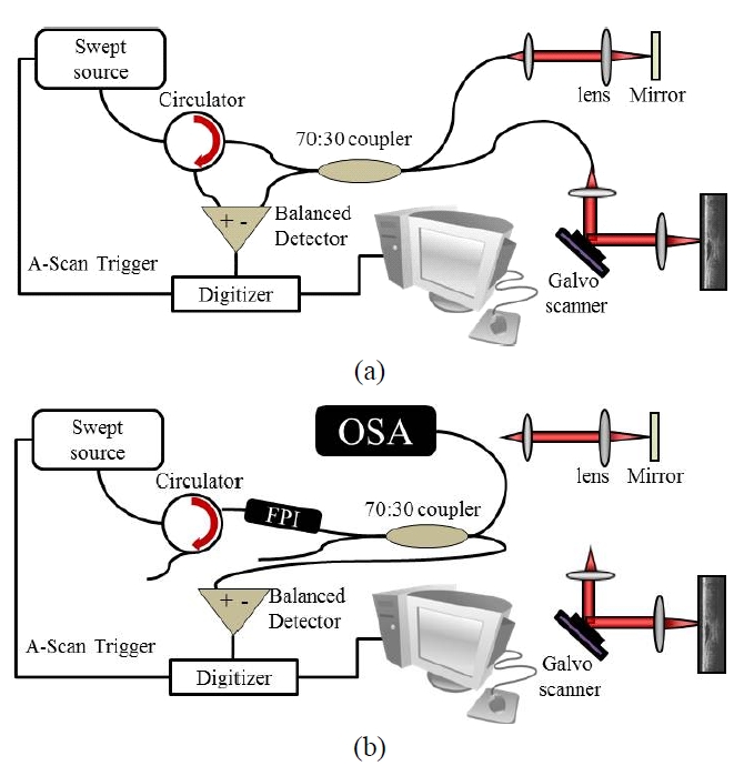
       2.1. Experimental Hardware Setup

    The swept source used in this study is HSL-2000 (Santec Co.) without the k-trigger function. Its center wavelength is 1329 nm with full width half maximum (FWHM) of 110 nm, and maximum sweeping rate of 20 kHz. A balanced photo detector has the electrical bandwidth of DC-100 MHz and the optical bandwidth of 800 to 1650 nm. A fiber-based FPI and an optical spectrum analyzer (OSA) are used for the generation of the two arrays. For the case using the output of the FPI, the OSA primarily increases the sample points for linearization or compensates the unstable output of the FPI, which contains noise. A schematic diagram of the fabricated OCT system is shown in Figure 1. Figure 1(a) is the structure of the fabricated SS-OCT system. A galvanometer scanner in the sample arm and a high-speed digitizer with a 100 MHz sampling rate are used for two dimensional (2D) imaging. The processing time difference for linearization in the k-domain is compared by using two different processing units; Nvidia Geforce GTX260 GPU and Core 2 Quad 2.4 GHz CPU. Figure 1(b) shows the location of the FPI and the OSA for acquiring the interference signal to generate two arrays. The FPI is connected to the input of the optical coupler, whereas the OSA and photo-detector are connected to the outputs of the optical coupler. We could obtain the interference signal and its wavelength information at the same time. The phase stability of the sweep trigger of the light source is an important consideration in our method because the actual wavelength value in each temporal position from the photo-detector should be consistent over each imaging to maintain reliable k linearization performance. The instability is compensated by using a temperature stabilized Fiber Bragg Grating (FBG) sensor which reflects light with a constant wavelength, and the intensity pulse induced by the reflection triggers the start of each A-scan acquisition.

       2.2. Generation of k-triggering Linearization Arrays

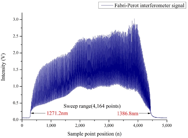
    First, we connected the FPI and the OSA to the fabricated OCT system as shown in Figure 1(b). After that, we generated a linearized wave number pattern with the same number of sample points as is acquired from the system. The measured wavenumbers corresponding to the peak locations from the output signal of the FPI are searched. The intensity signal correspond to one sweep acquired from OSA can be expressed as in Equation 1.

    image

    In this equation, λ is the wavelength and I(λ) is the intensity profile of the FPI output measured by the OSA. The change of wavelength corresponds to one step in A-scan signal, which depends on the optical resolution of the OSA, and the intensity change depends on the output signal from the FPI, measured simultaneously.

    The output signal of the FPI acquired from the photo-

    detector can be expressed as in Equation 2.

    image

    Here, t is the time, I(t) is the intensity of the FPI and tn depends on the sampling frequency of a digitizer. All intensity changes in the equations (1) and (2) are followed by the output signal of the FPI. In this case, the spectral compositions from FPI and OSA are not consistent each other per each A-scan because of variations up the instability of the source and noise condition. Therefore, information from OSA can be used as a reference position for the unstable FPI outputs. So, from the signal obtained from the OSA, we can transform the wavelength of the start and end positions of the effective spectrum to the wave-number (k). Figure 2 shows the FPI output signal from the light detection part. In this result, the minimum and maximum wavelengths measured from OSA in the sweep region are 1271.2 nm and 1386.8 nm, respectively. The number of sample points is 4164 in the sweep region. So, we transformed minimum and maximum values to the wave-numbers, and generated the linearized wavenumber line by linearization fitting as the same number as for the sample points.

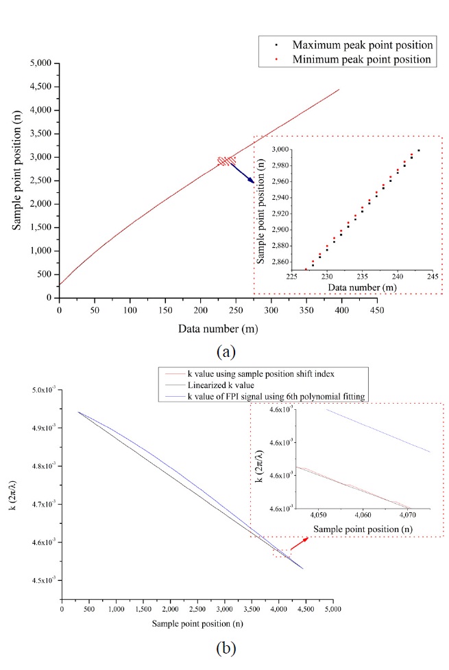
    Then, the low frequency component in the FPI output signal is removed by using a high pass filter, and the index is generated by detecting the peak intensity in each period. Because the index has constant interval information of wavenumber, we generated a wavenumber array by interpolation using 6th order polynomial fitting with the same number of sample points as the original.

    Based on the linearized wavenumber, we searched for the closest location of wavenumber in the interpolated wavenumber array. The difference between two wavenumber locations was saved in another array. This shift array of sample points is used as a lookup table hereafter, so we can perform linearization of the wavenumber by readjusting OCT signal position without any other linearization process.

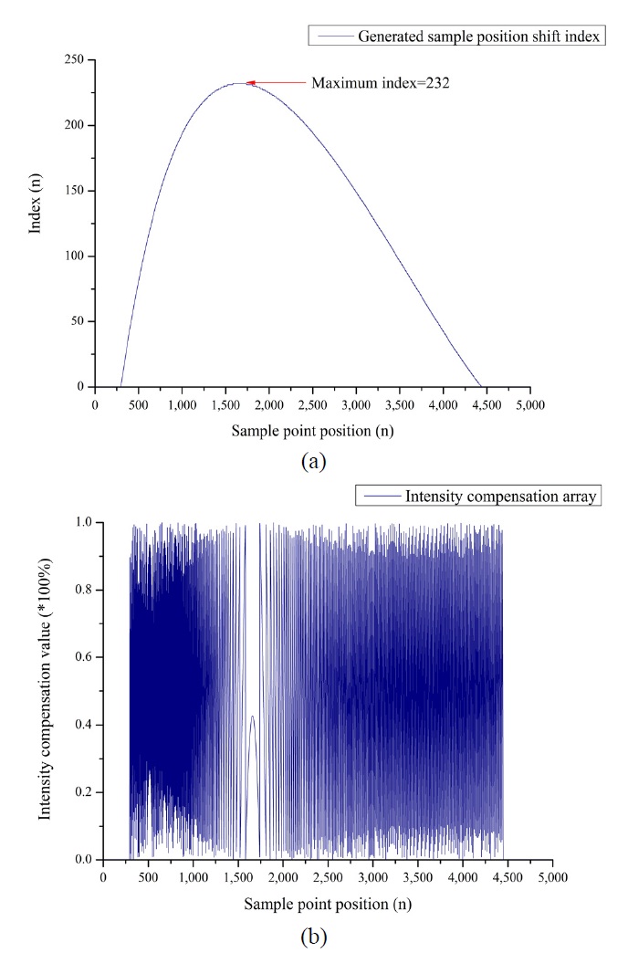
    When we use the method of searching for the approximate wavenumber, there can be discrepancy in the intensity proportional to approximated wavenumber. So, to compensate this error, we generated an intensity compensation array that can adjust the intensity proportional to the approximate wavenumber difference. We modified the OCT intensity with the intensity compensation array when moving to the wavenumber linearization location. This intensity compensation array is generated just one time when the calibration is performed. After that, when the output image appears in a display, all locations of OCT signals and intensities are compensated by the lookup table. So, we dramatically increased the output speed because there is not an additional com-pensation algorithm for each OCT A-scan output.

    In the FPI output signal from fabricated SS-OCT system, the index peak corresponding to every periodic peak signal is generated by using a peak detection algorithm, and detected indices are the minimum and maximum locations of the peaks. The number of detected index is 396 and the result is shown in the figure 3(a). After that, we determined

    the variation of wavenumber Δk among the peak to peak value of 792 points and generated the interpolated wave-number array from the determined wavenumber and detected index using 6th order polynomial fitting with the same number of sampling points as the original. The determined wavenumber value is shown in figure 3(b). The blue line is the interpolated wavenumber array using the polynomial fitting, and the black line is the array by linear fitting.

    The sample position shift index is generated to provide information of the amount of the shift to the most appro-ximate linearized wavenumber by comparing the acquired wavenumber array and the computed linearized wavenumber array. If the number being searched for between two wavenumber values is equal or less than the corresponding linearized wavenumber value, the closest measured wave-number value is selected in our method. The generated sample position shift index is shown in figure 4(a) and the maximum sample point is 232 points. The shifted and

    linearized values with only sample position shift index are shown in figure 3(b) as a red line. This result shows that it is inevitable that there is difference between measured and linearized wavenumber when we find the approximate wavenumber. So the nonlinearity remains to a certain level. In the case of using the hardware trigger, there is also some nonlinearity because of electrical noise and variable frequency fluctuation.

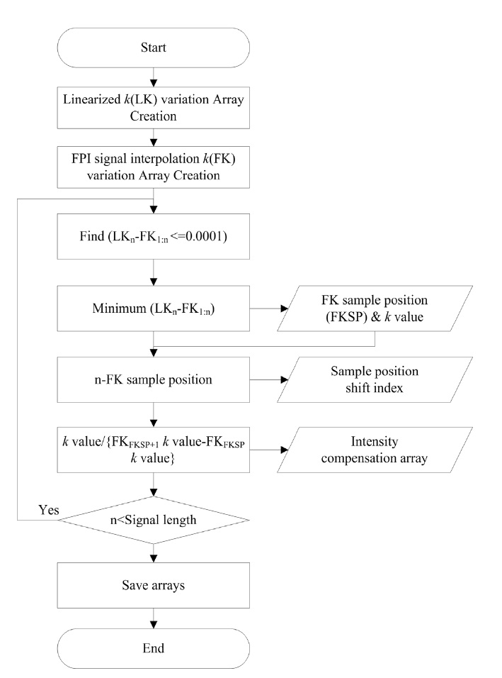
    We generated the intensity compensation array wavenumber to compensate residual nonlinearity. Difference from approxi-mation is calculated in the entire sweeping region when a sample position shift index is generated. So it is not necessary to recalculate in the OCT imaging program. If we divide the difference from approximation to the difference between current and next sample point position, we can calculate the mismatch of wavenumber as less than unity. In the OCT imaging software, if we multiply the acquired interference signal by the calculated intensity difference and the intensity compensation array, the mismatched wave-number value is compensated. The generated intensity com-pensation array is shown in figure 4(b). The two arrays are generated by using Matlab 2009b (The Mathworks. Inc.) and the flowchart of the array generation program is shown in figure 5.

       2.3. Experimental Protocol

    We verified performance enhancement with the generated sample position shift index and intensity compensation array by evaluating PSF and SNR in each A-scan, and SNR and CNR in the B-scan image of the IR sensing card.

    The PSF is acquired from the interference pattern by moving the mirror with a step of 500 μm in the sample arm of the fabricated SS-OCT, and SNR is calculated at each movement position with and without the intensity compensation array. The image of IR sensing card is obtained at optical path length difference of 2.5 and 6.0 mm, and from that, we calculated the SNR and CNR value with and without the intensity compensation array.

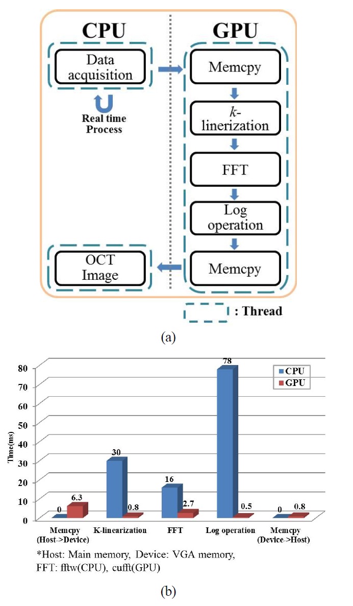
    Finally, we measured the processing time with the two arrays to the OCT software in two cases when the main processor of program is CPU and GPU. The program is coded with the C++, four multi-threads are used for data acquisition, signal processing, imaging and image saving. In the case of using GPU as a main processor, we only used GPU for signal processing in the multi-thread structure.

    III. EXPERIMENTAL RESULTS AND DISCUSSION

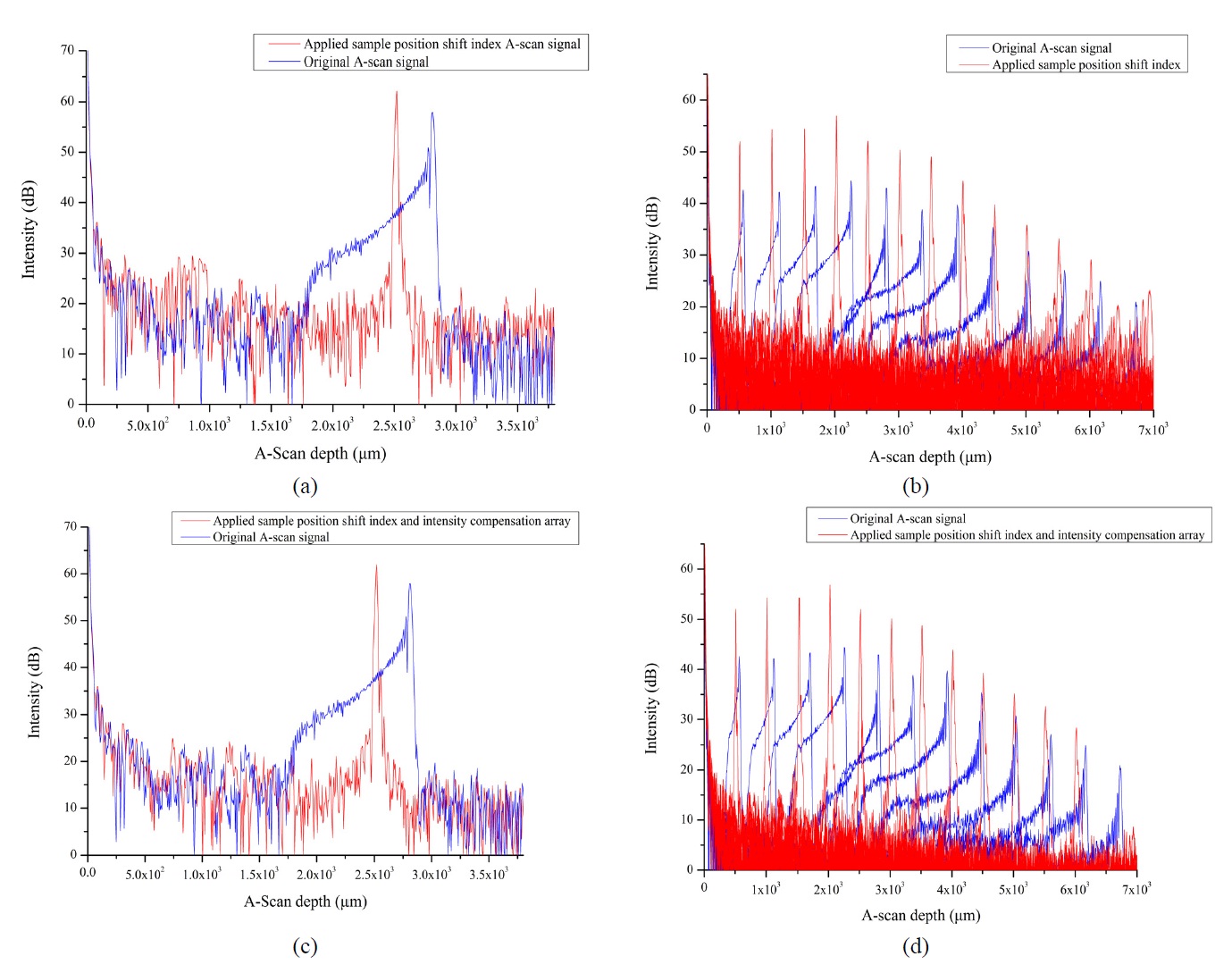
    Figure 6 shows linearized results for A-scan signal at 2.5 mm depth and the difference among the PSFs at variable depth. The A-scan signal of a mirror in 2.5 mm depth is shown in the figure 6(a), (c) and measured PSFs from 0.5 to 6 mm depth as a step of 0.5 mm are shown in figure 6(b), (d). Figure 6(a) and (b) are only applied to sample position shift index, and figure 6(c) and (d) are applied to both sample position shift index and intensity compensation array. In the cases using only sample position shift index like figure 6(a) and (c), they showed better noise characteristics at 2.5 mm depth than others. Especially, in the case of figure 6(b) and (d), the noise level was dramatically increased in the PSF when the depth is deeper than 4 mm. In the case of using only sample position shift index, it showed maximum SNR of 55.39 dB in PSF shown in figure (6). And in the case of using both the sample position shift index and intensity compensation array, it showed maximum SNR of 61.08 dB. There was a performance enhancement from 1.76 to 9.7 dB in measured SNR at each depth. It means that the compensation of nonlinearity can show more effective result in the deeper region.

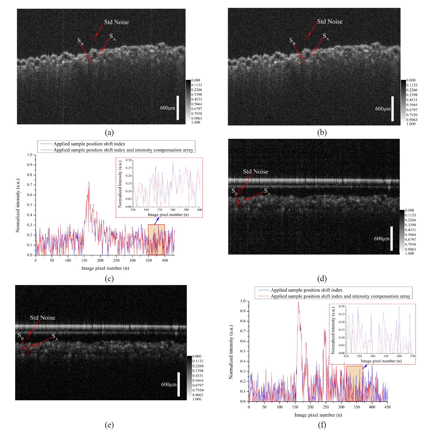
    We measured the IR sensing card at optical path length difference of 2.5 and 6.0 mm to recognize the difference at the output image. To exclude the effect of lens focal length at the sample arm, we just modified the optical

    path length of the reference arm and the result is shown in figure 7. Figure 7(a), (b), (c) are images of IR sensing card at optical path length difference of 2.5 mm, and figure 7(d), (e), (f) are at the 6.0 mm,. Figure 7(a), (d) are only applied to sample position shift index, and figure 7(b), (e) are applied to both the index and the array. The image size of IR sensing card is 512×431 pixels at 2.5 mm difference, and 300×451 pixels at 6.0 mm. At this time, the number of sample points is 5000. Figure 7(c) and (f) are the A-scan results correspond to 256 line number in each image. At marked area in figure 7(a) and (b), the CNR values are 4.54 and 4.63 which are increased by 0.09, respectively. Also, the SNR was increased from 32.27 to 32.73 dB by 0.04 as shown in figure 7(c). It is just small enhancement, but noise is decreased about whole image of IR sensing card. And the signal to background noise is stable in overall image. In the result at optical path length difference of 6.0 mm, there was an enhance-ment of 1.44 than the case of using the index only. Also, the SNR was increased by 1.29 dB in the 256 line number as shown in figure 7(f). Especially, like the result of the IR sensing card image at optical path length of 6.0 mm, the optical path length shows certain difference. So, the SNR was much decreased by 27 dB. But in the case which is applied to both the index and array, the CNR value was maintained as the level of 4.67. The theoretical/ measured axial resolutions are calculated to be 4.96 μm and 7 μm, respectively. The dispersion is not further compensated in these values.

    We measured the time required for imaging output software of fabricated SS-OCT when we use the main processing unit as CPU and GPU, and the result is shown in figure 8. The data size for the measurement is 5000 (FFT size)*300(A-scan). The structure of signal processing using GPU is shown at figure 8(a). We designed so that all threads except for acquiring data and displaying the output images are processed at GPU. When we use CPU as a main processor, the working threads corresponding to GPU are realized by multi-threads based on CPU. In this case, the time required for data acquisition is 47 ms, which is able to realize real-time imaging. The measured time is shown in figure 8(b) and the application of GPU can overall enhance the whole system performance. The entire time required for our linearization method of k-triggering is 30 ms for the CPU processing and 0.8 ms for the GPU processing, respectively. The real-time imaging is feasible in both cases. The entire time required for signal processing is 124 ms for the CPU processing and 11.1 ms for the GPU processing.

    The proposed linearization method using two arrays in k-triggering has a few merits. First, there is no optical power loss because optical components for generation of the com-pensation array are removed after the calibration step assuming stable light source and sweep trigger timing. Second, all computations for linearization are performed only during array generation. After then, a residual process is just movement among memory addresses. So the interpolation algorithm is not necessary in post signal processing. this can decrease the time required for imaging, so real-time imaging can be realized. Lastly, compensation performance for nonlinearity depends on sample point location, wave-length information, and proper algorithm, so it can be applied to all FD-OCT. Also it can be compensated by another interpolation algorithm for a highly nonlinear light source.

    IV. CONCLUSION

    We could confirm that just moving the sample point position and applying an intensity compensation array can compensate imprecision in wavenumber value. The perfor-mance is analyzed in aspects of SNR and CNR results. And the effect is increased as optical path length increases. This fact is more useful for the industry applications that needs inside information such as a structure or a volume surrounded with transparent materials, not just OCT appli-cation for biological tissues whose sizes are below 2 mm. Also, in the case of using an Axicon lens that can maintain the field of depth until a far distance without change of beam profile, the proposed method can be applicable for compensation of wavenumber mismatch.

    Based on our result, over 10 frames/s by CPU processing and 100 frames/s by GPU processing are realized for real-time imaging. Our linearization method is applicable to compensate unstable k-triggering performance in any swept source. Even if any hardware k-triggering is not supported, our method can be realized for the linearization in k-triggering by inserting the FPI or FBG just once in the calibration step.

    The proposed method is effective and powerful because it uses only two index arrays and they can compensate complex nonlinearity due to external generation of the array. And it is also suitable for real-time imaging due to its short processing time using any processor, CPU or GPU.

참고문헌
  • 1. Huang D., Swanson E. A., Lin C. P., Schuman J. S., Stinson W. G., Chang W., Hee M. R., Flotte T., Gregory K., Puliafito C. A., Fujimoto J. G. (1991) “Optical coherence tomography” [Optics and Spectroscopy] Vol.254 P.1178-1181 google cross ref
  • 2. Fercher A. F. (1996) “Optical coherence tomography” [J. Biomed. Opt.] Vol.1 P.157-173 google cross ref
  • 3. Fercher A. F., Drexler W., Hitzenberger C. K., Lasser T. (2003) “Optical coherence tomography-principles and applications” [Rep. Prog. Phys.] Vol.66 P.239-303 google cross ref
  • 4. Choma M. A., Hsu K., Izatt J. A. (2005) “Swept source optical coherence tomography using an all-fiber 1300-nm ring laser source” [J. Biomed. Opt.] Vol.10 P.044009 google cross ref
  • 5. Xi J., Huo L., Li J., Li X. (2010) “Generic real-time uniform k-space sampling method for high-speed swept-source optical coherence tomography” [Opt. Express] Vol.18 P.9511-9517 google cross ref
  • 6. Gelikonov V. M., Gelikonov G. V., Shilyagin P. A. (2009) “Linear-wavenumber spectrometer for high-speed spectral-domain optical coherence tomography” [Optics and Spectroscopy] Vol.106 P.459-465 google cross ref
  • 7. Ding C., Bu P., Wang X., Sasaki O. (2010) “A new spectral calibration method for Fourier domain optical coherence tomography” [Optik] Vol.121 P.965-970 google cross ref
  • 8. Vergnole S., Levesque D., Lamouche G. (2010) “Experimental validation of an optimized signal processing method to handle non-linearity in swept-source optical coherence tomography” [Opt. Express] Vol.18 P.10446-10461 google cross ref
  • 9. Jeon M., Kim J., Jung U., Lee C., Jung W., Boppart S. A. (2011) “Full-range k-domain linearization in spectral-domain optical coherence tomography” [Appl. Opt.] Vol.50 P.1158-1163 google cross ref
  • 10. Wang Z., Yuan Z., Wang H., Pan Y. (2006) “Increasing the imaging depth of spectral-domain OCT by using interpixel shift technique” [Opt. Express] Vol.14 P.7014-7023 google cross ref
  • 11. Eigenwillig C. M., Biedermann B. R., Palte G., Huber R. (2008) “k-space linear Fourier domain mode locked laser and applications for optical coherence tomography” [Opt. Express] Vol.16 P.8916-2937 google cross ref
  • 12. Azimi E., Liu B., Brezinski M. E. (2010) “Real-time and high-performance calibration method for high-speed sweptsource optical coherence tomography” [J. Biomed. Opt.] Vol.15 P.016005 google cross ref
  • 13. Yasuno Y., Hong Y., Makita S., Yamanari M., Akiba M., Miura M., Yatagai T. (2007) “In vivo high-contrast imaging of deep posterior eye by 1-μm swept source optical coherence tomography and scattering optical coherence angiography,” [Opt. Express] Vol.15 P.6121-6139 google cross ref
  • 14. Gora M., Karnowski K., Szkulmowski M., Kaluzny B. J., Huber R., Kowalczyk A., Wojtkowski M. (2009) “Ultra highspeed swept source OCT imaging of the anterior segment of human eye at 200 kHz with adjustable imaging range” [Opt. Express] Vol.17 P.14880-14894 google cross ref
  • 15. Potsaid B., Baumann B., Huang D., Barry S., Cable A. E., Schuman J. S., Duker J. S., Fujimoto J. G. (2010) “Ultrahigh speed 1050nm swept source/Fourier domain OCT retinal and anterior segment imaging at 100,000 to 400,000 axial scans per second” [Opt. Express] Vol.18 P.20029-20048 google cross ref
  • 16. Zhang K., Kang J. U. (2010) “Real-time 4D signal processing and visualization using graphics processing unit on a regular nonlinear-k Fourier-domain OCT system” [Opt. Express] Vol.18 P.11772-11784 google cross ref
  • 17. Watanabe Y., Itagaki T. (2009) “Real-time display on Fourier domain optical coherence tomography system using a graphics processing unit” [J. Biomed. Opt.] Vol.14 P.060506 google cross ref
  • 18. Van der Jeught S., Bradu A., Podoleanu A. Gh. (2010) “Realtime resampling in Fourier domain optical coherence tomography using a graphics processing unit” [J. Biomed. Opt.] Vol.15 P.030511 google cross ref
OAK XML 통계
이미지 / 테이블
  • [ FIG. 1. ]  (a) Schematic diagram of the OCT system, (b) Schematic diagram of k-linearization component setup.
    (a) Schematic diagram of the OCT system, (b) Schematic diagram of k-linearization component setup.
  • [ FIG. 2. ]  FPI output signal intensity with sample point position of k-linearization component setup.
    FPI output signal intensity with sample point position of k-linearization component setup.
  • [ FIG. 3. ]  (a) Sample point position of minimum peak and maximum peak using peak detection algorithm, (b) Linearized k value at minimum to maximum k using linear fitting (Black line), k value of FPI output signal using 6th order polynomial fitting (Blue line) and k value of resampled FPI output signal using sample position shift index (Red line).
    (a) Sample point position of minimum peak and maximum peak using peak detection algorithm, (b) Linearized k value at minimum to maximum k using linear fitting (Black line), k value of FPI output signal using 6th order polynomial fitting (Blue line) and k value of resampled FPI output signal using sample position shift index (Red line).
  • [ FIG. 4. ]  (a) Generated sample position shift index at full sample point position, (b) generated intensity compensation array at full sample point position using compared k value with linearized k value and k value of resampled FPI output signal.
    (a) Generated sample position shift index at full sample point position, (b) generated intensity compensation array at full sample point position using compared k value with linearized k value and k value of resampled FPI output signal.
  • [ FIG. 5. ]  Flow chart of k linearized sample position shift index and intensity compensation array using MATLAB.
    Flow chart of k linearized sample position shift index and intensity compensation array using MATLAB.
  • [ FIG. 6. ]  Point spread function, (a) and (c) are A-scan results using two arrays at 2.5 mm depth, (b) and (d) are PSFs results at 0.5 mm step different depths using two arrays.
    Point spread function, (a) and (c) are A-scan results using two arrays at 2.5 mm depth, (b) and (d) are PSFs results at 0.5 mm step different depths using two arrays.
  • [ FIG. 7. ]  IR sensing card image at optical path length difference 2.5 mm and 6.0 mm , (a) and (b) are IR sensing card images at 2.5 mm, (d) and (e) are IR sensing card images at 6.0 mm, (c) and (f) are compared A-scans k linearization results using the sample position shift index and the intensity compensation array.
    IR sensing card image at optical path length difference 2.5 mm and 6.0 mm , (a) and (b) are IR sensing card images at 2.5 mm, (d) and (e) are IR sensing card images at 6.0 mm, (c) and (f) are compared A-scans k linearization results using the sample position shift index and the intensity compensation array.
  • [ FIG. 8. ]  Comparison of system processing time between CPU and GPU, (a) is the process structure using GPU, (b) is compared to process time of GPU and CPU.
    Comparison of system processing time between CPU and GPU, (a) is the process structure using GPU, (b) is compared to process time of GPU and CPU.
(우)06579 서울시 서초구 반포대로 201(반포동)
Tel. 02-537-6389 | Fax. 02-590-0571 | 문의 : oak2014@korea.kr
Copyright(c) National Library of Korea. All rights reserved.