Recently, a great deal of attention has been focused on the bio-technology field and its applications which extend the life-span of human beings. Along with this trend, biological flow has also attracted the interest of researchers in the field of fluid engineering. Optical methods have been employed in many of the dominant measurement systems due to the rapid advances in optics as well as the wide variety of applications of the method. For example, particle image velocimetry (PIV), generated by using several optical systems, implements the scattering light image of a particle illuminated by a laser light sheet [1]. Conventional laser Doppler velocimetry (LDV) is another optical method for measuring flowing fluid, although, it is a single-point measurement method with limitation in the single point measurement of flow [3].
In particular, optical tomographic techniques are important in the medical field, because these techniques can provide non-invasive diagnostic images. This is achieved by generating slice images of three-dimensional objects [4]. Basically, optical coherence tomography (OCT) utilizes a low coherence Michelson interferometer to obtain high-resolution crosssectional imaging of biological tissues [5-7]. By using OCT, the human retinal inner structure, including the cellular tissue layer, has been digitized. In general, MRI and CT modalities are not suitable for examining those areas with a high resolution [2]. With the advantages of a non-invasive tissue structure image scanning method, OCT is used to monitor blood glucose concentration of patients with diabetes based on the correlation between OCT signal slope and glucose concentration [8].
The OCT system is advantageous in the synthesis of crosssectional images and can show in depth the biological tissue structure by detecting small changes in the backscattered light. Generally, the conventional OCT records only the amplitude of light reflected as a function of depth within tissues. Therefore, as the more effective technique from the fluid dynamic point of view, the optical Doppler tomography (ODT) system, which is the functional extension of OCT, has been suggested and proven to obtain exceptionally useful imaging modality for many biological applications [9-12]. The ODT system utilizes the basic optical principle of OCT. In addition, it can simultaneously obtain the velocity information of a moving object that goes through the system and the structure image of biological tissue by measuring the amplitude and phase of the interference fringe intensity generated between the reference and the sample arm [13,14]. Comparing with other fluidic measurement systems such as PIV and LDV, ODT can show the micro-scale cross-sectional images of the inner tube and the fluidic information simultaneously. By using two-axis scanning, it has overcome LDV’s limitation as well as enabling the construction of 3 dimensional fluidic volume images.
To evaluate ODT system performance, the velocity profile in a capillary tube is measured based on the variation of fluid flow rate. The algorithm used in this study as well as the results can serve as a novel method to measure flow velocity profile in an opaque annulus such as a blood vessel for biological applications in fluid dynamics. In this paper, an SD-ODT system was applied to detect the cell depletion layer and to observe dynamics of the RBCs of blood.
II. EXPERIMENTAL APPARATUS AND METHOD
2.1. Doppler Frequency Shift and Basic Algorithm
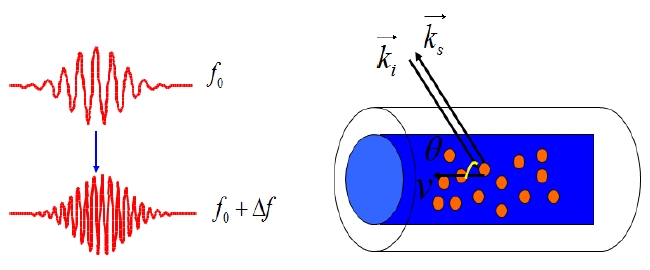
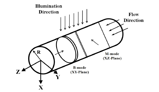
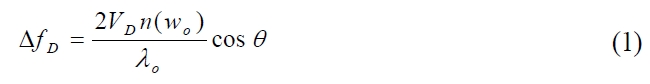
Optical Doppler techniques are based on the interference phenomenon of light scattering caused by the interference of moving particles with a reference beam [4]. When the seeding particles flow through a channel at a constant velocity, as shown in Fig. 1, the backscattered light signal from the particles contains a Doppler frequency component. This is different from the incident illumination beam light signal mainly because of the difference in the path lengths between the two signals. By detecting the frequency shift component, the relative flow velocity can be analyzed with a proper conversion algorithm at the post processing stage. It is known that the shift is linear in the velocity and its amplitude depends on the angle between the sample beam and the flow [15]. Therefore, the Doppler frequency shift
value is obtained by detecting temporal interference as
where
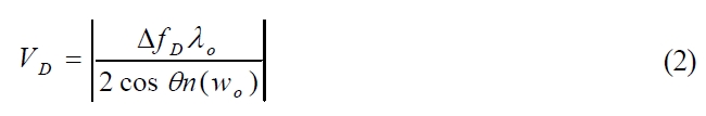
Based on the above Doppler effects, we can implement the ODT system to measure the flow velocity profile inside a channel.
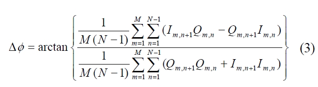
The frequency shift induced by the motion scattered in the direction of the incident laser beam can be estimated using the Kasai autocorrelation function [16]. The Kasai autocorrelation function measures phase shifts between two adjacent A-scans. It can be derived using Eq. (3):
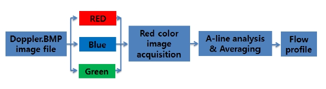
A standard Doppler color-map is used where red indicates the flow in the direction of the optical beam while blue indicates flow in the opposite direction in the images (Fig. 2). The maximum detectable phase shift without aliasing is ±π, due to the complicated blood flow profile and the presence of noise. Thus, no attempt is made to phase-in the unwrapped
images. Furthermore, due to the difficulty in determining the Doppler angle in the complicated structures of blood vessels, we did not relate the phase shift to the velocity of the moving scatterers [17].
2.2. Experimental Setup and Measurement System
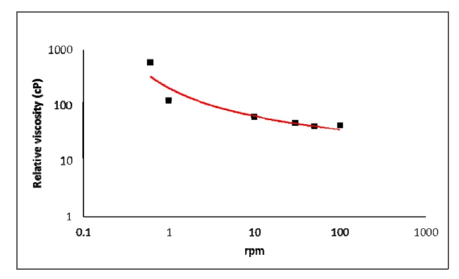
Unadulterated mouse blood samples are obtained from 20 mice. To measure the viscosity of blood, a rotational viscometer (LVDV?II+Pro ; Brookfield Engineering, USA) is employed and the temperature is maintained at 26℃. A shear stress is related with the force component parallel to the streamwise flow velocity component. From the fluid dynamic view point, the component of shear stress is the product of the fluid viscosity coefficient and the shear rate for a flowing fluid, the velocity gradient of the fluid. Consequently, we can approximate the flow motion, i.e. fluid element deformation, based on shear rate variations in the fluid flow. The shear rate increases proportionally to the increment of the revolution rate. Figure 3 shows relative viscosity variations of blood according to the increase of spindle revolution in the ranges from 0.3 to 100 rpm. From the relative viscosity distribution, shear-thinning characteristics of blood flow are clearly identified.
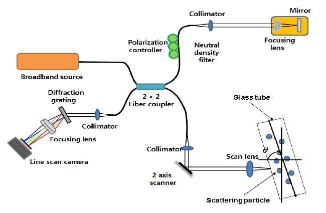
A schematic diagram of the spectral-domain optical coherence tomography (SD- OCT) system used in the current study is shown in Fig. 4. The SD-ODT system consists of interferometers based on fiber-optics. The SD-ODT light source is a super luminescent emitting diode (SLED) centered at 840 nm with full width at half maximum (FWHM) of 80 nm. The SLED light is split into two fibers by a 2 × 2 (50:50) fiber coupler, and the fibers are directed to the reference arm and sample arm of the interferometer. The spectrometer is composed of a diffraction grating, collimator, and achromatic doublet lens. The interference signal from the interferometer is acquired by 12-bit line scan CMOS camera with 2048 pixels (Basler Sprint spL2048-140k, Germany). The camera drives with maximum line rate of 140 kHz, 1080 MHz camera line clock and vertical binning mode. Images are acquired by PCIe-1429 frame grabber (National Instruments, USA). The galvo-scanner (Cambridge technology) was used in the sample arm and analog input/ output (PCI-6731; National Instrument) was used to drive the scanner.
In the sample arm, the light was focused by an objective lens with a focal length of 40 mm. The light that was backscattered from the sample is coupled back into the optical fiber. When the optical path length difference between the sample and the reference arms are minimized within the
coherent gate, interference fringes can be observed at the detection path.
A glass capillary tube with 120 μm inner diameter is placed perpendicularly underneath the probing light. We prepared the three capillary tubes to reveal the effect of different concentrations of HR. One tube serves as the control. To make the control solution, we used the scattering particle solution, prepared by mixing warm water (65.9℃) and creamer (19 g). The two other tubes contain different concentrations of HR (5%, 25%).The solution flow in a capillary tube is driven by a syringe pump (HARVARD APPARATUS, accuracy +/- 0.5%, maximum flow rate 7.909 ml/min., minimum flow rate 0.0014 μl/hr) at constant flow rates of 900 μm/s, 1100 μm/s, and 1300 μm/s. From the display information of the syringe pump, the initial flow rate condition can be checked easily and the capillary tube inlet center velocity can be obtained by dividing the corresponding cross-sectional area.
Three different capillary tube inlet flow velocities (vinlet) were tested in the present study. The values of vinlet were 900 μm/s, 1100 μm/s, and 1300 μm/s. The Reynolds number (Re), which is based on the capillary tube inner diameter, ranges from Re=6 to 48 [18]. Reynolds number is normally used to identify flow characteristics as a measure of the ratio of inertial forces to viscous forces. Consequently, at low Reynolds number, such as in the microfluidic domain, viscous forces are dominant and the flow is characterized by smooth fluid motion. To measure the velocity component, we set Doppler angle (
Figure 5 shows the coordinates used in this experimentation. Blood flows along the axis of channel. M-scan and B-scan are two dimensional images for the XZ-plane and XY-plane. The laser light, travelling in the +X direction, illuminates the top of the channel and produces an angle of 80 degrees with the flow direction.
3.1. M-scan and B-scan OCT/ODT Images Aquisition
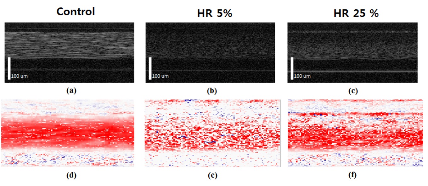
Figure 6 shows longitudinal-section (XZ-Plane, Y=0) images under the different conditions in a 120 μm glass tube by the M-scan. The top and bottom rows are OCT and ODT images respectively. Three types of conditions were used - water seeded with white powder, HR 5% blood, and HR 25% blood. We seeded white powder in order to visualize water since the SD-ODT system cannot detect clear water.
Good images were obtained from the whole blood. We added Phosphate buffered saline (PBS) solution to dilute the whole blood. The cell depletion layer was obtained easily at lower HR rate. In the OCT and ODT images, different points between HR 5% and HR 25% were observed. Based on the OCT and ODT images, we could observe different thicknesses of cell depletion layers clearly according to HR variations between 5% and 25%. In addition, we can easily conjecture the velocity distribution of blood flow with the axial migration feature from these two images. Velocity variations in the diluted blood flow in the central region were observed. These are shown in Figs. 6 (e) and 6 (f). The variations can be attributed to the presence of cells, mostly red blood cells, in the blood flow. In the case of the control, as shown in Fig. 6(a), we achieved a laminar flow and nearly uniform velocity distribution in the channel center region (Fig. 6(d)). ODT images show specific color for each velocity. More intense red means faster velocity. Velocity information is saved as vector data.
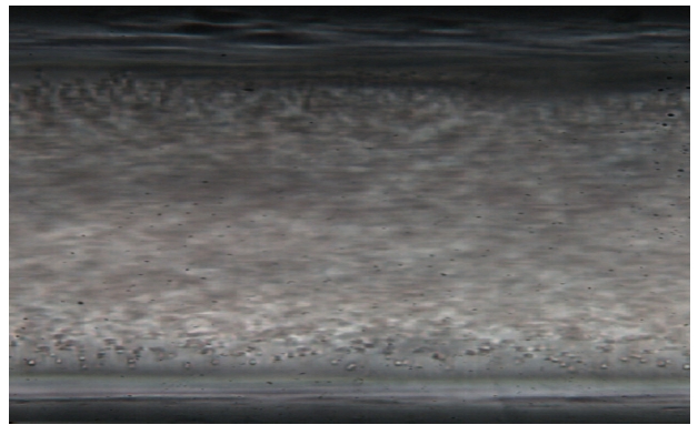
We measured the cell depletion layer in the blood flow using the SD-ODT system. In a small capillary less than 300 μm in diameter, the cell depletion layer is a near-wall layer of plasma without RBCs. In general, the RBCs all migrate to the center of the blood vessel. This is shown in Fig. 7. This phenomenon indicates aggregation (RBCs unite for efficient moving) or changing of viscosity (RBSs change through deformation of their shapes; thus their viscosities vary to reduce the increasing shear stress close to the blood vessel wall). The size of the cell depletion layer is determined through the blood flow velocity and HR. Moreover, in the HR 20%, the cell depletion layer exists below 3 μm in the blood vessels or micro-channels [19].
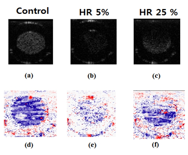
Figure 8 shows cross-sectional images in B-mode (XY Plane, Z=0). The HR 5% and HR 25% images contain the distribution profiles of RBCs. We tried to observe the existence of the cell depletion layer in the channel wall in different viewing points. In addition, we expected to observe the layer around the channel wall in cases of HR 5% and HR 25%. However, the cell depletion layers were not clearly observed. ODT images show velocity profiles according to colors, either red or blue. The profile close to the circle center is displayed in blue: the profile farther from the circle center is indicated in red. We calculated the velocity profile and created graphs which are shown in Fig. 9.
In the current study, the size of the cell depletion layer cannot be measured with data and pictures. The main reason is the limited resolution of the SD-ODT system. Despite the effort of experimenting with a variety of parameters (decreased HR and faster flow velocity), results were inconclusive. However, we found that the SD-ODT system is advantageous in measuring the velocity field compared with the other systems mentioned in the introduction.
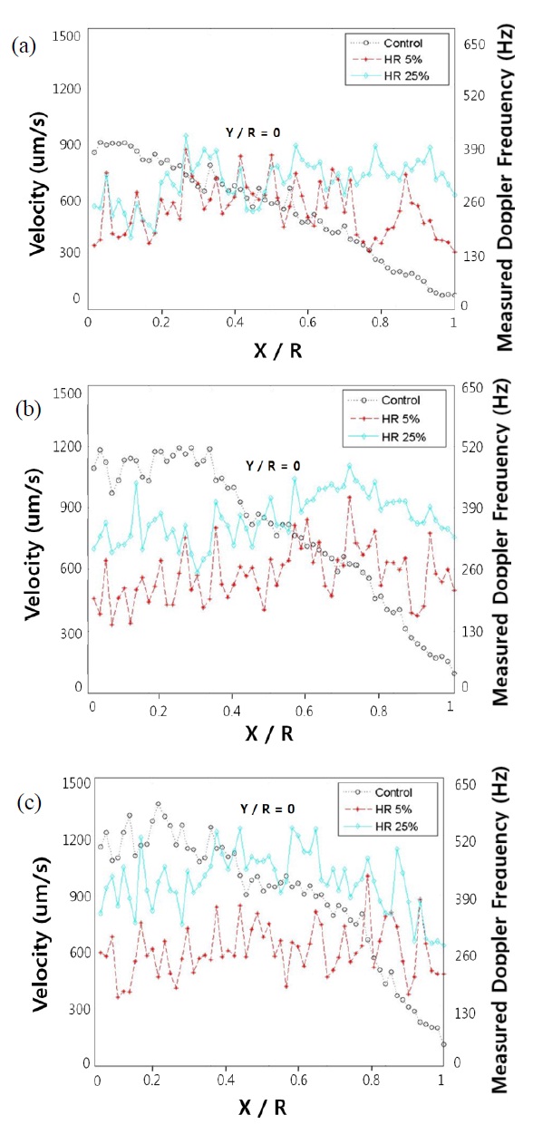
3.2. Flow Profile Measurement for the Three Different Flow Velocities
In Fig. 9, our calculations of the flow velocity and Doppler frequency profiles measured in the depth direction of a glass capillary tube at the Doppler angle of 80 degrees are
shown. Each graph corresponds to the different flow velocities of 900 μm/s, 1100 μm/s, and 1300 μm/s. With the assumption of a symmetric profile, the half region from the central axis to inner surface of the capillary tube was considered. We calculated a Doppler shift of the power spectrum of the temporal interference fringes with Kasai autocorrelation function. To obtain the actual Doppler frequency shift induced by the flow, the background shift information at a null velocity was used as the baseline velocity profile. The null velocity implies that there is no flowing motion in any direction, except for the Brownian motion of small seeded particles. When a specific flow in the tube is induced, the actual Doppler frequency shift caused by the flow is obtained by subtracting the null velocity profile baseline from the flow measurement. All of the control mode graphs are shown as Gaussian shapes. Thus, these systems could measure the exact velocity of fluid in flow. In the profile of blood velocity flow, the graphs show different shapes compared with the control. Blood can change viscosity according to the position. Blood is known as a shearthinning fluid and as such, most of the cells naturally migrate to the central region of blood vessels [20]. Therefore, the velocity of blood flow in the channel wall region at the mid-height is accelerated due to the shear-thinning feature of blood. In addition, the profile has relatively blunt shape compared with the control. Furthermore, blood consists of RBCs, WBCs, and so on. These components counteract each other.
As a result, the SD-ODT systems could not detect the cell depletion layer in the present study. Nevertheless, these systems were proven to be capable of observing the RBCs of blood. Using the SD-ODT system is a non-invasive method. As a future work, experimentation can be conducted in vivo based on the developed SD-ODT system.
The mouse blood flow inside a capillary tube was investigated experimentally using the SD-ODT system. Comparative analysis was performed with the results using white powder under the same experimental condition. The flow structure of diluted mouse blood is markedly different from that of white powder. The use of the SD-ODT system for blood flow investigation is advantageous particularly in non-invasive medical examination.
The captured flow images of particles in the control (white powder) and blood cells in HR 5% and HR 25% demonstrate good quality and velocity tracking-ability. However, the blood flow showed less velocity variation in the channel in the central region due to the presence of numerous blood cells in mouse blood. The stream-wise velocity of blood flow achieved larger values in the region near the channel wall due to the shear-thinning feature of blood. The velocity profile showed relatively blunt shapes compared with those of white powder. The SD-ODT system used in the present study can overcome the single-point measurement limitation by scanning the interesting region in sequence at a short period in the depth direction. From these results, the SD-ODT system can be used to obtain reliable and in depth flow velocity profiles.