Flutter boundary prediction during wind tunnel and flight tests is one of the most important, but very difficult tasks imposed in the process of development of a new airplane (Bisplinghoff, et al., 1955; Fung, 1955). Flutter boundary prediction methods in which only measured wing response signals are analyzed can be classified into two categories:

A. Damping approach based on measurement of the damping coefficient of flutter mode,

B. System stability approach based on the estimation of stability of an aeroelastic system.

The category B is further classified into two subcategories:

B1) Flutter margin for continuous-time systems (FMCS) (Poirel et al., 2005; Price and Lee, 1993; Zimmerman and Weissenburger, 1964) based on Routh’s stability test,

B2) Jury’s stability criterion defined in the discretetime domain (Matsuzaki and Ando, 1981; Matsuzaki and Torii, 1990), and the flutter margin for discrete-time systems (FMDS) (Bae et al., 2005; Torii and Matsuzaki, 1999, 2001) founded on the Jury criterion.

The first category A is very traditional, and it is still very popular in practical applications in spite of its intrinsic difficulties. As clearly seen in Fig. 1 of an experimental study (Irwin and Guyett, 1968) published late in the 1960’s, the damping coefficient of the flutter mode often reveals two problems in a critical speed-range very close to the flutter boundary:

a) Rapid change in its value, that is, suddenly decreasing and becoming zero, as seen both in analyses and experiments of the so-called explosive flutter,

b) Large scattering of its measured values in experiments.

As for the second difficulty b), a more-recent survey (Koenig, 1995) on the results of 16 different flutter tests pointed out that there was a scatter of about 30% in the damping coefficient while only 3% in the corresponding frequency.

To compensate the first difficulty a), a criterion for a twomode system which was characterized by a gradual change, named flutter margin (FMCS-2), was proposed (Zimmerman and Weissenburger, 1964). FMCS-2 is based on Routh’s stability test in the continuous-time domain, and is expressed with measured frequencies and damping coefficients of the first two modes. Therefore, FMCS-2 also spreads widely due to the second problem b) mentioned above. To account for uncertainty caused by the scattering, two stochastic approaches (Poirel et al., 2005) were introduced in estimating FMCS-2. The stochastic analysis, However, the stochastic analysis cannot improve the accuracy itself in the prediction of the critical boundary. An extended criterion for a threemode flutter (FMCS-3) was also proposed (Price and Lee, 1993).

Hereafter, we will focus on Subcategory B2, that is, the flutter boundary prediction based on the stability criteria defined in the discrete-time domain, because digital techniques have enormously developed for the last two decades. Therefore, we may now apply easily the modern estimation and identification methods to data analysis of measured responses to estimate flutter characteristics in a subcritical range. In other words, it is possible that the flutter margin, modal frequencies and damping coefficients are estimated accurately from certain duration of the response even contaminated with inevitable noises, including mechanical and electric ones.

The present overview is a revised version of the author’s paper (Matsuzaki, 2011b), which was up-dated from the original (Matsuzaki, 2011a) by referring to a couple of recent publications and including the Section 5.

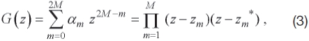
In the discrete-time domain, the advanced counterpart of Routh-Hurwitz’s stability criterion (Fung, 1955) in the continuous-time case is Jury’s stability criterion being developed from the one first established by Schur-Cohn (Jury, 1964). Like the Routh-Hurwitz condition, Jury’s criterion is defined in terms of the coefficients of the characteristic equation of the system, as will be described later. Needless to say, once characteristic coefficients are estimated from sampled measured data, not only stability but also the dynamic characteristics of the system, such as the modal frequencies and damping coefficients, can be evaluated at the same time.

Early in 1980’s, the present author and his coworker (Matsuzaki and Ando, 1981) proposed an innovative approach for predicting the flutter boundary based on Jury’s stability criterion together with an autoregressive movingaverage (AR-MA) representation for sampled random responses. Applying it to a flutter test of a cantilever wing model performed in a transonic wind tunnel, they showed that the Jury criterion was much more eff ective in predicting the flutter boundary than the damping coefficient of the flutter mode. This criterion was also successively applied to the prediction of divergence boundary of a forward-swept wing tested in a supersonic wind tunnel (Matsuzaki and Ando, 1984). Two decades later, a new stability parameter for a two-mode flutter, named "flutter margin for discretetime systems" (FMDS-2) (Torii and Matsuzaki, 1999, 2001), was derived from the Jury criterion. The new parameter is mathematically equivalent to FMCS-2 in the continuoustime case, provided that the sampling period is suffi ciently short (Torii, 2002; Torii and Matsuzaki, 2001). FMDS-2 was recently extended to FMDS-3 for a three-mode flutter (Torii and Matsuzaki, 2011). An extension of FMDS-2 to a multimode flutter (FMDS-N) (Bae et al., 2005) was also proposed to apply with success to a wind tunnel test of a wing with a fl ap. However, FMDS-N in the case of the two-mode does not agree with the original FMDS-2, as pointed out in Matsuzaki (2005). Recent numerical studies (Hallissy and Cesnik, 2011; McNamara and Friedmann, 2007) showed that FMDS-N did not work well as a predictor of flutter onset for multi-mode wing systems.

The AR-MA process for a sampled signal of random responses, Jury’s stability criterion and three versions of FMDS, i.e., FMDS-2, FMDS-3, and FMDS-N, will be briefly summarized.

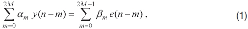
It is assumed that the stationary response, y(t), of a wing flying at a fixed speed in an atmosphere with a Gaussiantype turbulence of a given variance, is sampled at a constant interval T to produce a sequence of random variables, {y(kT), or simply written, y(k); k=1, 2, …, N}. The stationary random sequence is assumed by an AR-MA model (Goodwin and Sin, 1984) as

where α₀=1 and α_2M≠0. The order 2M, AR coefficients {αm} and MA coefficients {βm} with m=1, …, 2M, are an unknown integer and real numbers to be estimated from the sampled data, {y(k)}. A sequence, {e(k); k=1, …, N-1} represents noise inputs to the system, that is, a Gaussian independent random sequence with zero mean and an unknown variance σ². Application of the z-transform (Jury, 1964) to the left-hand side of Eq. (1) yields the characteristic equation:

where

and z_m^*(m = 1, 2, ... , M) stands for a complex conjugate of z_m. It is obvious that M represents the number of the modes consisting of the aeroelastic system. The eigenfrequencies, ω_i, and the damping coefficients, η_i, of the i-th mode are respectively given as

Jury’s criterion (Jury, 1964) is defined by

where X_i and Y_i are i x i determinants whose elements are one of the AR coefficients or zero. The dynamic and the static instability, namely, flutter and divergence of the system with M degrees of freedom is respectively given by

The flutter margin for a two-, three-, or multi-mode system (FMDS-2 [Torii and Matsuzaki, 2001], FMDS-3 [Torii and Matsuzaki, 2011], or FMDS-N [Bae et al., 2005]) is respectively expressed as

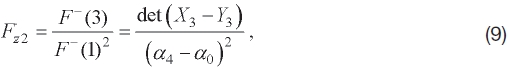
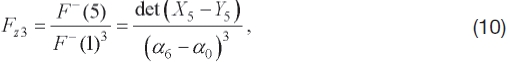
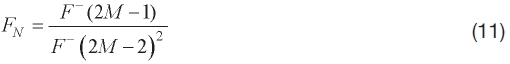
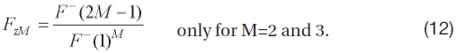
From Eqs. (9) and (10), we have a unified formula (FMDS-M for M = 2 and 3):

It is proved (Torii, 2002; Torii and Matsuzaki, 2001) by using the Tustin transform that FMDS-2 is mathematically equivalent to FMCS-2 in the continuous-time domain, provided that the sampling period T is suffi ciently short. FMDS-N defined by Eq. (11) in the case of M = 2 does not agree with FMDS-2 given by Eq. (9).

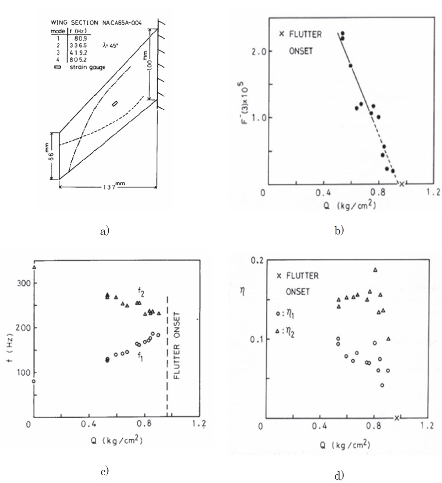
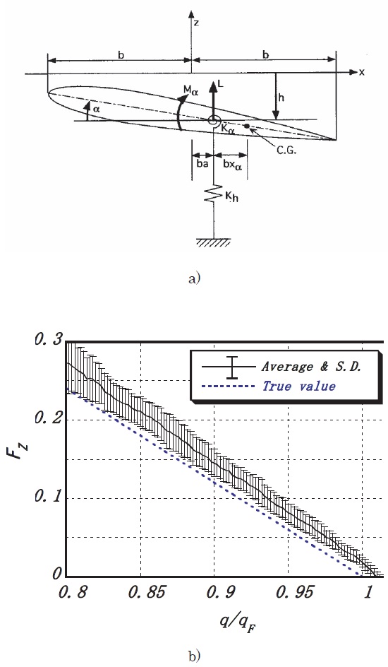
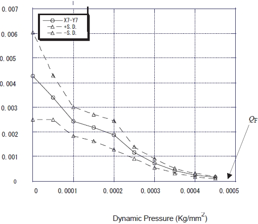
The first application of Jury’s stability criterion to a flutter test was made by using a cantilever wing model, as shown in Fig. 1a, tested at Mach number 1.17 in a transonic blow-down type wind tunnel (Matsuzaki and Ando, 1981). During the test, at each blow the dynamic pressure was kept constant for about ten seconds and to measure the response of the wing randomly excited by natural flow turbulences. The response at each blow was stationary, because its mean value and standard deviation remained essentially the same with time, more accurately its covariance was the same. The measurement was repeated by increasing the dynamic pressure stepwise. As the flutter criterion, the parameter F^-(3)=0, obtained by setting M=2 in Eq. (7), was applied to measured data which had been band-passed to contain contributions mainly from the first two modes. In Fig. 1b, evaluated values of F?(3) are shown by solid circles against the dynamic pressure, Q, between about 0.5 and 0.9 kg/cm². The flutter boundary was predicted to be about Q= 0.95 kg/ cm² by fitting a straight line to the solid circles given only between about 0.5 and 0.8 kg/cm², and by extrapolating the fi tted line to cross a point on the horizontal coordinate, which was close to the experimental value (Q_F = 0.97 kg/cm²) given by a cross on the coordinate. In Figs. 1c and d, the modal frequencies, f₁ and f₂, and the damping coefficients of the first two modes, η₁ and η₂, calculated respectively by using Eqs. (4) and (5) are plotted by circles and triangles at

the same pressures as for F^-(3) shown in Fig. 1b. It is clearly very difficult to predict the boundary simply by using the damping coefficients, as seen in Fig. 1d.

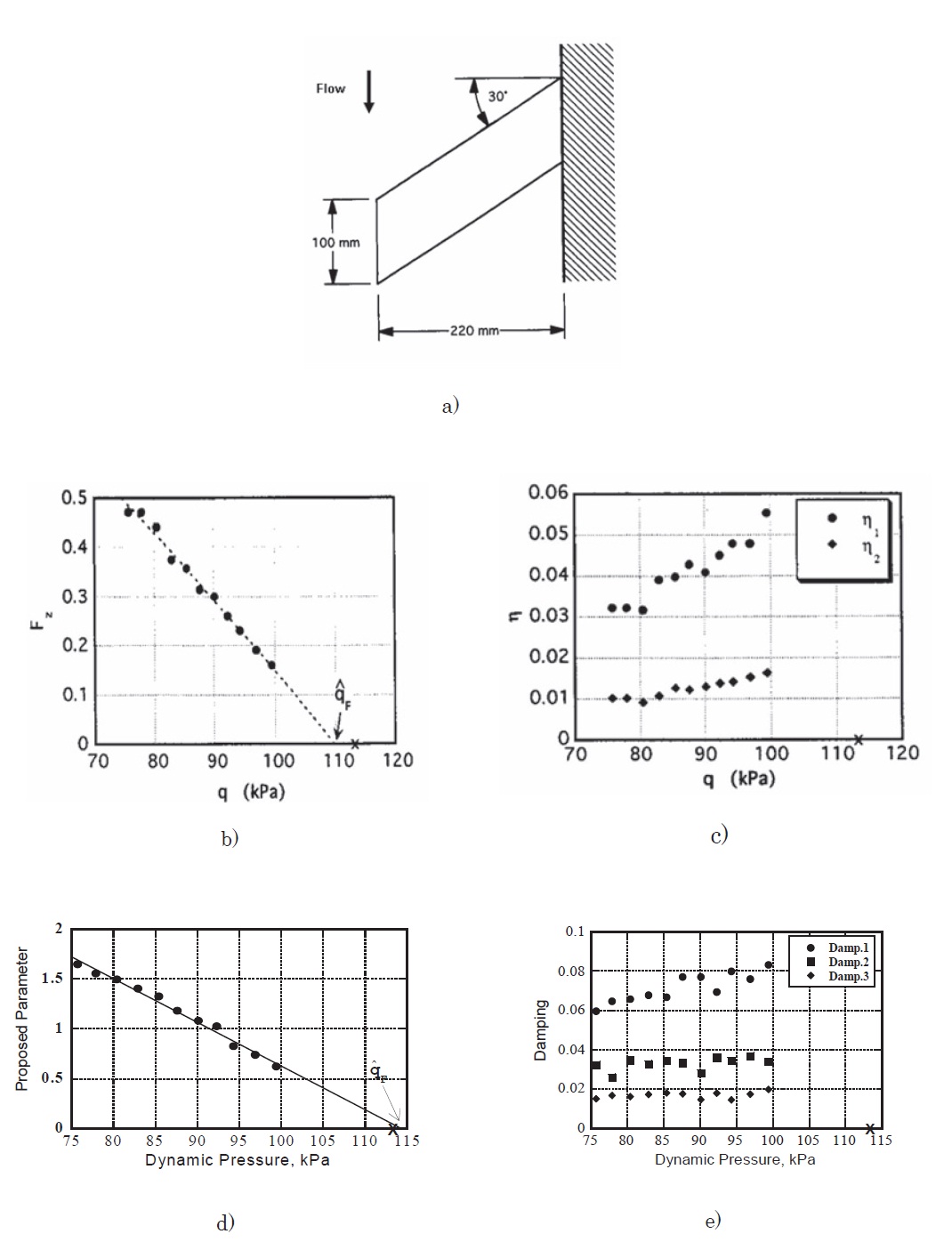
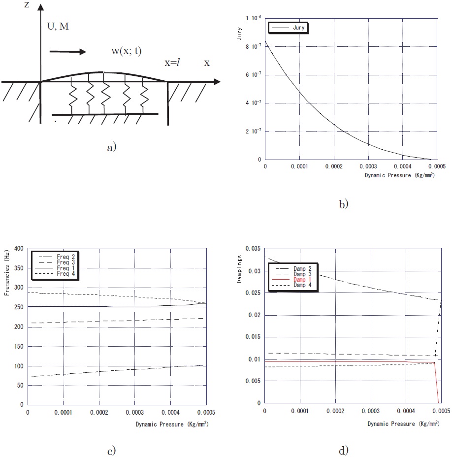
Figures 2b-e show numerical results obtained by applying the approach based on FMDS-M to experimental data of a wing model shown in Fig. 2a, which were measured at M = 2.51 at a supersonic wind tunnel. FMDS-2 and FMDS-3 were, respectively, applied to sampled sequences obtained by band-passing the measured data so as to contain mainly the responses due to the first two modes (Torii and Matsuzaki, 2001) and due to the first three (Torii and Matsuzaki, 2011). In Figs. 2b and d, estimated values of FMDS-2 and FMDS-3 are plotted by solid circles in the pressure range up to q = 100 kPa, with the measured flutter boundary, q_F = 113.5 kPa, shown by a cross on the horizontal coordinate. A dotted and a solid straight line are fitted to the circles shown below q = 100 kPa and extended to cross the horizontal coordinate at a point representing an estimated boundary,

located very close to the cross on the coordinate. The calculated damping coefficients, η₁ and η₂, are also given up to q = 100 kPa in Fig. 2c and η₁, η₂ and η₃ in Fig. 2e. In these figures, again, it is not possible to predict the boundary shown by the cross by using the estimated damping coefficients. It is clear that FMDS-M for M = 2 and 3 is effective in predicting the flutter boundary

from a low dynamic pressure range. The effectiveness of the flutter margins was also analytically confirmed by using the so-called two-dimensional simple wing without and with a flap, that is, with two and three degrees of freedom, respectively.

As for a four-mode system (M = 4) of a cantilevered wing with a flap (Bae et al., 2005), the extended parameter F_N defined by Eq. (11) was used to predict its flutter boundary in a test. Figure 3 shows a comparison between the application of F_N during the test and the flutter analysis by the U-g method. F_N decreases linearly to find the boundary at 832 Pa. In the U-g diagram, there are two curves of g which cross the horizontal coordinate. With a small amount of structural damping, for example, g = 0.02 being taken into account in this figure, the critical point given by the fourth mode at 717 Pa would shift at about 1,000 Pa. However, the other crossing point at about 800 Pa due to the second mode would move to around 830 Pa to give the flutter boundary. Hence, agreement among the U-g approach, the prediction by F_N and the experimental value of the boundary was good.

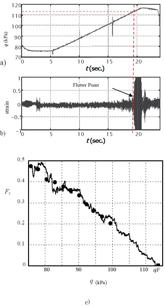
To determine the flutter boundary in a single test, the dynamic pressure was often increased at a fixed rate until it arrived at its critical value (Matsuzaki and Ando, 1985; Torii and Matsuzaki, 1997, 2002). Figures 4a and b illustrate time histories of the dynamic pressure which increased from 76 to

117 kPa and the signal of a strain gage glued on the surface near the root of the same wing as used for the stationary test and shown in Fig. 2a. The standard deviation of the response signal increased gradually with time, and the wing suddenly started to flutter at q_F= 113.5 kPa (Torii and Matsuzaki, 2002), as mentioned in Section 3.1. For the prediction of the flutter boundary, sequential data sampled from the strain signal shown in Fig. 4b were assumed in a nonstationary AR-MA process, and its coefficients were evaluated through the

use of recursive maximum likelihood estimation technique (RMLE) (Ljung, 1987), since they were time-dependent. In Fig. 4c, recursively estimated values of FMDS-2 are plotted by a wavy solid curve against the dynamic pressure up to the flutter point given by a solid square on the horizontal coordinate. The fluctuation of the estimated values was sufficiently small except for a low pressure range, say, below 85 kPa, where the estimation was not well converged around the true values because RMLE had started with a set of initial values arbitrarily selected. In the nonstationary case, FMDS- 2 was again almost linearly decreased over the range up to q_F = 113.5 kPa except below 85 kPa. For comparison, numerical values of FMDS-2 of the stationary test, like those shown in Fig. 2b, are also given by solid circles, which lie mostly on the curve. Before the wing model was broken during the nonstationary test, the stationary test was first performed to measure the stationary responses

To exploit and confirm analytically the feasibility of the system stability method, the author and his co-researcher performed numerical simulations by using the twodimensional simple wing with only two degrees of freedom in an incompressible flow, or by introducing a panel system supported with a distributed spring and exposed to a supersonic flow. In these studies, the generalized theory of unsteady aerodynamic forces (Edwards, 1977) was used to generate responses of the wing and the panel in an arbitrary motion caused by random air turbulences.

Like in Section 3.2, nonstationary responses of the twodimensional simple wing, shown in Fig. 5a, exposed to a turbulent flow whose dynamic pressure increased at a fixed rate, were represented by the AR-MA process, and its coefficients were evaluated by using RMLE. The evaluation of the response was repeated fifty times by using a different sequence of flow turbulence. Figure 5b shows the mean and standard deviation of evaluated values of FMDS-2, respectively, by a solid line and a small I-shaped column against the dimensionless pressure, q/q_F, from 0.8 to 1.02 (Torii and Matsuzaki, 2002), although the evaluation was made from q/q_F = 0, where q_F stands for the flutter boundary. A dotted line, named "True value", represents FMDS-2 of a flutter analysis, being redrawn from a part of the curve shown, for instance, in Fig. 4 of Torii and Matsuzaki (2001), where FMDS-2 decreased in a linear manner from q/q_F = 0 to 1.0. FMDS-2 may, therefore, provide a good tool to predict the

flutter boundary for the nonstationary process, too, because its mean value changed nearly in a linear manner. It is noted that, because of a dynamic effect due to the nonstationary process, the flutter boundary shifted to 1.02 from 1.0 of the true value obtained in the flutter analysis, as shown in Fig. 5b.

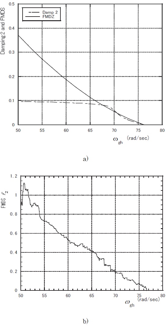
The recent development of morphing aircraft technology has now presented a new-type of technical problems. Among them, aeroelastic instability is one of the most challenging issues (Lee and Weisshaar, 2005; Tang and Dowell, 2008). In an ordinary airplane the flight speed is the most visible variable to the instability. In other words, the higher the flight speed is, the more critical the stability becomes. On the other hand, as for the morphing wing, we may consider that, even though the flight speed is kept fixed, the wing will onset flutter in the process of morphing in which the structural adaptation happens to lead to a "coalescence" of the frequencies of aeroelastic modes of the wing. In other words, the morphing technology presents a new type of nonstationary process. Accurate measurement of modal damping coefficients is considered to be harder in such nonstationary situations. Applicability of the nonstationary approach, mentioned in Sections 3.2 and 4.1, to a simple morphing wing was studied (Matsuzaki and Torii, 2005, 2006, 2007) by assuming that the stiffness of the wing shown in Fig. 5a was representatively given by the natural frequencies of the heaving and the pitching motion, ω_gh and ω_gα, and that the morphing mechanism was influential only on the stiffness, namely, the two natural frequencies of the wing. In a numerical simulation of morphing, only ω_gh increased continuously at a constant rate with ω_gα being fixed.

In Fig. 6a, numerical results of the flutter analysis, that is, FMDS-2 and the damping coefficient of the critical mode, η₂, are plotted against ω_gh from 50.0 to 80.0 rad/sec, respectively by a solid and a chained line, while ω_gα was kept at 100 rad/ sec. As ω_gh increased from ω_gh = 50 rad/sec, FMDS decreased uniformly and became zero at ω_gh.cr = 76.2 rad/sec. On the other hand, η₂ remained almost unchanged up to about ω_gh = 69 rad/sec, and then started to decrease rapidly to zero at ω_gh.cr. Figure 6b illustrates numerical results of the nonstationary simulation analysis in the morphing process, in which ω_gh increased at a constant rate of 0.5 rad/sec per second. The coefficients of the nonstationary AR-MA process were again estimated by RMLE. FMDS-2 decreased almost linearly in a range from above ω_gh = 55 rad/sec and became zero at ω_gh = 76.5 rad/sec, which was higher than ω_gh.cr due to the effect of the dynamic process. It was confirmed (Matsuzaki and Torii, 2012) that FMDS-2 was useful in predicting the flutter boundary, ω_gh.cr, of the morphing wing from a sufficiently lower range of ω_gh.

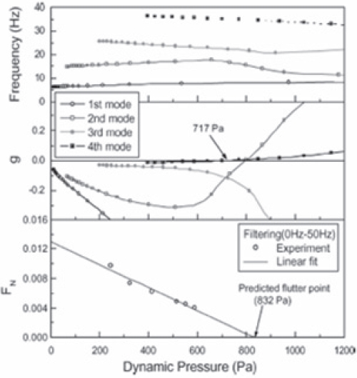
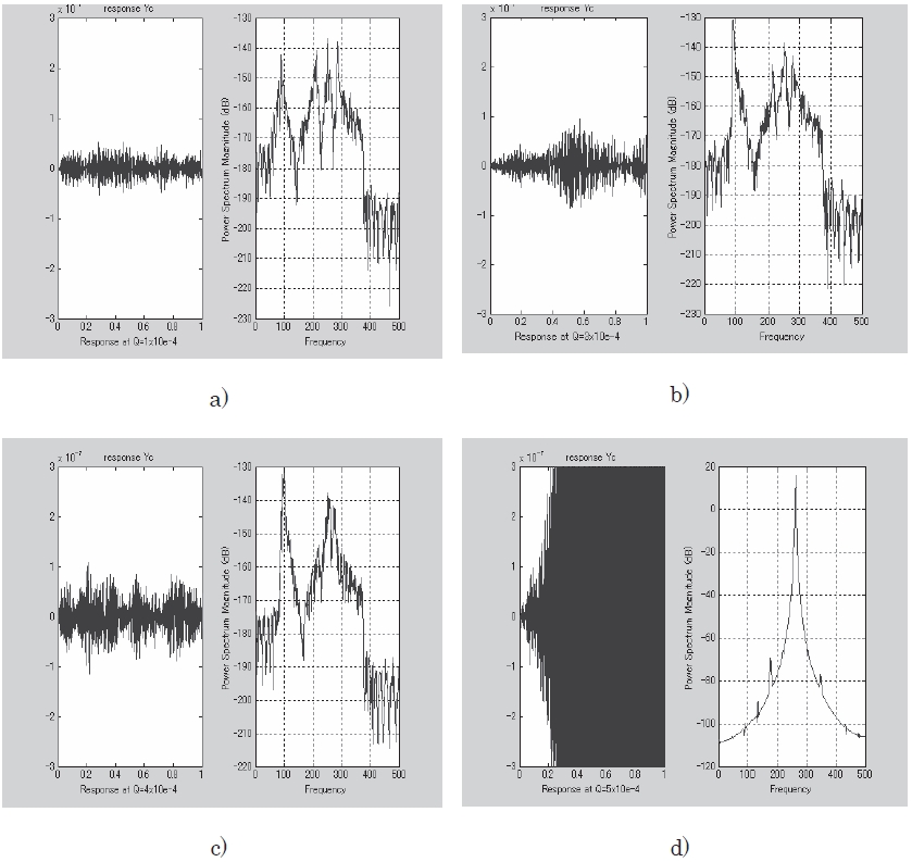
Airplane wings with auxiliary airfoils or additional attachments encounter often aeroelastic instabilities involved with a higher-order mode. A very flexible wing of a high-aspect ratio became critical also due to an involvement of a high-order mode (Hallissy and Cesnik, 2011). In order to develop systematically the flutter boundary prediction applicable to a multi-mode flutter, numerical simulation analyses (Matsuzaki, 2009, 2010) were performed by utilizing responses of a panel which was supported with a distributed spring and exposed to a supersonic flow, as shown in Fig. 7a. As is well-known, the onset of panel flutter does not usually lead to an immediate destruction of the panel structure, so that the prediction of the flutter boundary is less serious than

in wing flutter. The reason for using the panel system is that we may easily create an aeroelastic situation in which the two modes intentionally designated are coupled to induce flutter, and that the two-dimensional quasi-steady supersonic flow approximation is applicable as a generalized unsteady theory (Edwards, 1977) to generate the panel response caused by air turbulence. Furthermore, the responses of the panel obtained in a subcritical speed resembled very much those of a wing model often observed during a wind tunnel test, as will be seen later. For this multi-mode system, it is assumed that the value of an effective spring constant of the i-th mode, k_i, is selectable arbitrarily, so that proper adjustment of the spring constants makes it possible to cause flutter due to an aeroelastic coupling between the two designated modes. As

the first step, the four-mode system was analyzed, in which four different couplings between (Case I) the first and the second mode, (II) the second and the third, (III) the third and the fourth and (IV) the first and the fourth were examined. Results of flutter analysis on Case IV, that is, F^？(7)?X₇?Y₇, the modal frequencies and the damping coefficients of the four modes are shown against the dynamic pressure, Q, in Figs. 7b-d, respectively. The coupling between the first and the fourth mode is clearly seen in Fig. 7c. Jury’s parameter F^-(7) decreased more or less in a uniform manner to become zero at the flutter boundary, Q_F = 4.9× 10^?4 kg/mm². On the other hand, as shown in Fig. 7d, the damping coefficient of the first mode shown by a solid line kept its value very close to 0.01 up to about Q = 4.8× 10^?4kg/mm² and with a slight increase in

Q it quickly became zero at Q_F.

Based on this preliminary analysis, numerical simulations on flutter boundary prediction of the aeroelastic system were performed by assuming that the dynamic pressure increased in a stepwise manner. Figures 8 show time histories of panel response (Case IV) of one second at four dynamic pressures, that is, a) Q = 1.0× 10^?4, b) Q = 3.0× 10^?4, c) Q = 4.0× 10^?4, d) Q = 5.0× 10^?4 (kg/mm²). The responses shown in these figures are quite similar to those of wing models which we often observe during wind tunnel tests. As the critical pressure was Q_F = 4.9× 10^?4 kg/mm², the response diverged in an oscillatory manner in Fig. 8d. At ten dynamic pressures including these three Cases a) to c), F^?(7) was evaluated. In Fig. 9, the mean and the standard deviation of F^?(7) based on ten estimations at each dynamic pressure are given by a square and a pair of triangles. It is obvious that a simple extrapolation of a solid line connecting the squares will cross the horizontal coordinate at a point close to the boundary, Q_F, indicated

by an arrow. As for the remaining three cases, similar results were obtained.

Before discussing the matters related to the system stability approach, we note that the first application of the time-series representation of wing response was given by using the AR process in 1978 (Onoda, 1978), although the system stability was not taken into account in the analysis. A number of researchers used also the AR or the ARMA representation of wing responses in the 1980s and 90s, for example, Batill et al. (1992), Pak and Friedmann (1992), and Roy et al. (1986).

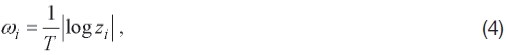
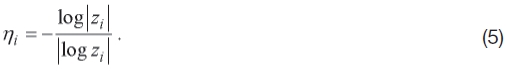
As discussed above, the flutter boundary prediction based on the system stability approach has great advantages due to advanced digital techniques, although the number of its applications is very small so far. For the present, it may serve as a complement to the damping method. This is because the latter approach has a very long history of practical applications and experiences, whereas the former needs to experience much more actual applications. Modern estimation methods supposedly allow us to eliminate much of noise effects from measured noise-contaminated data, and estimate sufficiently accurate system parameters. For this end, however, it is necessary to appropriately select initial input parameters for a computing program, such as the sampling period, T, the number of data, N, the upper and the lower limit of a band pass filter, f_U an f_L, etc., as well as specific parameters associated with the programs used. Some comparisons among estimated results of FMDS, modal frequencies, etc., obtained by changing input parameter values, were given, for instance, in Torii and Matsuzaki (1992, 1995, 2001). For the parameter calibration, the modal frequencies and damping coefficients directly measured in a test will also serve as useful references. The evaluation of Jury’s criterion, FMDS-M and FMDS-N is rather simple and easy, once the order 2M and the AR coefficients of the system have been estimated. In an actual application, it is recommended to evaluate all these criteria as well as the modal frequencies and damping coefficients given respectively by Eqs. (4) and (5).

Although Jury’s criterion, more specifically, F^?(2M?1) given by Eq. (7), is applicable to an aeroelastic system with any degrees of freedom, an effort for extension of the effective FMDS-3 to a flutter margin for higher-mode systems is important, because multiple frequencies of uncoupled modes may exist very close to or between the frequencies of the coupled modes. In such a case, it is impossible to filter the sequence of measured data into one which contains only three modes including the coupled two.

As is well-known, the damping approach is not so effective, particularly in the case of the so-called explosive flutter for which the critical damping coefficient starts to decrease quickly in a narrow range close to the boundary and becomes zero to induce a violent self-excited oscillation. An expert of an American aircraft-manufacturing company says that a half of dozen wing models are constructed for a wind tunnel test because they are often destructed by the onset of explosive flutter. Needless to say, direct measurement of the damping coefficients from a once-jerked and quicklydamped oscillation is easily influenced by air turbulence because turbulent flows change their characteristics from one instant to another. On the other hand, by using modern digital techniques which developed remarkably over the last couple of decades, we may analyze stationary and nonstationary random responses measured for certain period, and extract more reliable values of the system parameters from measured data.

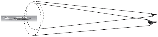
As for a wind tunnel test, from our past experiences although very limited, it seems that an ordinary wind tunnel provides sufficiently effective turbulences for the system stability approach. If the flow is calm, then one may install a vortex generator in an upstream of the test section to create required flow turbulences. On the other hand, as for a flight test in an open atmosphere, no one can expect any turbulence which will continue with the same strength for a sufficiently long range and a long period. However, recent development of unmanned aircraft technology is so remarkable that we may think of introducing a turbulence-generating system composing of a unmanned aircraft(s) equipped with a vortex generator(s), and also controlling the system to maneuver at a fixed distance ahead of a tested airplane and to produce air turbulence satisfying requirements in a region where the tested airplane flies. Figure 10 illustrates a schematic picture of flight test in which a vortex-generating system and a tested airplane fly together at a supersonic speed.

This paper presented an overview on the flutter boundary predictions based on the system stability approach for digitalized systems, that is, Jury’s stability criterion and flutter margin for discrete-time systems (FMDS-M and FMDS-N). The applications of the prediction method to a flutter system with multi-modes and to the nonstationary flutter test in which the dynamic pressure uniformly increased were mentioned. The extension of the nonstationary approach used for ordinary-type wings to the prediction of flutter of a morphing wing was reviewed, too.

Difficulties encountered by the traditional damping method and the system stability approach were discussed. Regarding a future application of the system stability method to flight test in an open air, a conceptual idea of a turbulencegenerating system composed of an unmanned aircraft(s) which flies at a fixed distance ahead of a tested airplane was proposed.