Sense and avoid is one of the most basic responsibilities for aircraft operations. Pilots who operate aircraft are always required to maintain a high level of situation awareness in order to avoid a mid-air collision. Increased traffic densities and large speed differentials in airspace can have high potentials for air collisions even in daylight and in visual flight rule conditions. Thus, an autonomous collision detection and avoidance capability is a critical capability for a variety of unmanned aerial vehicle applications in airspace. In order to aid pilots or autonomous flight computers much effort has been made in developing robust collision detection algorithms. Recent improvements in the field of image processing and computer vision have raised interest in the use of image sequences from passive optical sensors for detecting potential threats [1-5].
Most of the studies have been carried out by using a track-before-detect (TBD) technique and this technique, integrates the sensor data about a tentative target over time by combining target detection and estimation. Unlike other conventional detection techniques such as probabilistic data association (PDA) and multiple hypotheses testing (MHT), a signal is tracked before declaring it as a target. In the literature, TBD methods based on dynamic programming (DP) have been proposed for dim target detection and tracking in highly cluttered environments where the signal-to-ratio (SNR) is relatively low [1-6]. The DP-based TBD methods effectively integrate the observations along possible trajectories and those trajectories for which the tracking score exceeds a given threshold are returned as possible targets [6]. The DP solution proposed by Barniv is one of the first papers in the literature [1] that has provided a fundamental approach to detect and track dim moving targets simultaneously as registered in an image set. Arnold et al. [3] improved the existing solutions in terms of computational efficiency and performance against non- Gaussian noise characteristics. The analysis of the DP-based TBD was carried out by using extreme value theory in [6]. On the other hand, Nichtern et al. [7] dealt with some practical issues on setting the parameters of dynamic programming solutions in order to maximize the tracking capability. Although, there have been efforts to solve the various important TBD problems, the problem of developing track scoring functions has received less attention, particularly when it applies to airborne target detection on the flight path. As collision threats have a few geometric features from their relative dynamics, incorporating these features into track scoring functions is important to enhance the detection performance.
The fundamental technique presented in this paper is based on the DP solutions that were proposed in [1, 3]. However, our current work has led to some technical innovations in its application to the problem of airborne collision threat detection. In particular, a new track scoring function is proposed to improve the collision detection performance. This is done by reflecting two distinguishable properties of a non-maneuvering target in a collision course. First, a target on a near-collision course remains stationary in image view as collision occurs when the line-of-sight between aircrafts is maintained almost stationary. Second, the rate of image expansion for a collision course target is approximately inversely proportional to the time to collision [8]. As a result, the main problem of concern is in the development of a DP-based TBD technique that takes in to account these two properties for early airborne target detection.
This paper is organized as follows. In Section 2, the basic approach to DP-based TBD is described. Section 3 illustrates the development and implementation of a track score function of a DP solution for airborne target detection. Section 4 presents the numerical results and its performance assessment of the proposed method. The final section summarizes the overall discussion.
2. Dynamic Programming Solutions for Airborne Target Detection
The objective of airborne target detection is to determine the trajectories that are most likely to have originated from the actual threat by using the measured image sequence of
The DP-based target detection algorithm has been divided into three steps. In the first step, the raw image sequence passes through pre-processing stages. It emphasizes the potential targets and provides a four-dimensional target intensity measurement set with the spatial and velocity resolution cells. Spatial resolution corresponds to the image sensor resolution. The velocity resolution depends on the design parameter which is related to a three-dimensional data processing stage. In this step, a close-minus-open filter which is one of the morphological filtering algorithms is employed to extract peak regions in images and to generate a non-negative output [9]. The second step is the DP-based target detection stage that operates on the unthresholded data set that is provided by the pre-processing step. Basically, the DP approach provides a single optimization procedure that includes both data association and track detection as it avoids a thresholding process. Moreover, it also preserves all the signal information in the raw image data. The DP-based TBD method presented hereafter is based on the approaches that are described in [1, 3]. The final decision on the target presence and position is made in the third step by evaluating the criteria for both threshold values and uniqueness of track histories over a certain length of image frames.
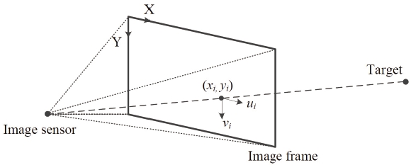
Target motion is modeled to be approximately linear over the image plane of an image sensor, with allowances for curvature, acceleration, and jitter. This model illustrates the target motion onto the image plane with the resultant target dynamics and it described two differential equations of motion as shown in Fig. 1. The target model is defined by a discrete-time state-space equation of the form,

Where, x
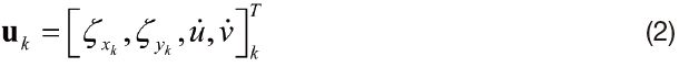
where ζ

and

are the unknown target acceleration components. The process noises are zero-mean Gaussian white noises with unknown statistics. The state transition matrix, F
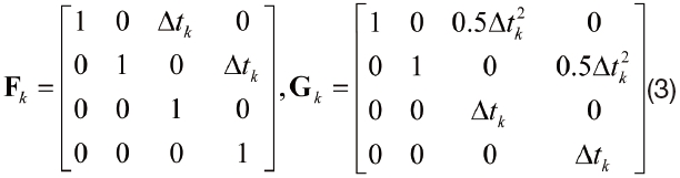
where Δ
The raw image data are pre-processed to suppress clutter signals prior to the dynamic programming stage. The threedimensional convolution filter is applied to brief image sequences for the extraction of the target’s expansion rate as well. Output from the image pre-processing step consists of discrete, four-dimensional matrices, Z
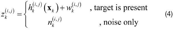
where
2.3 Dynamic Programming Solution
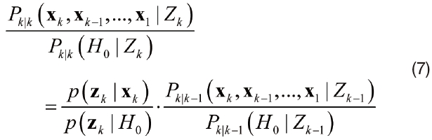
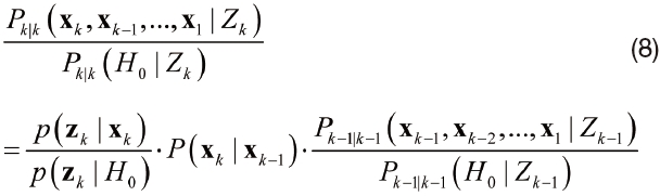
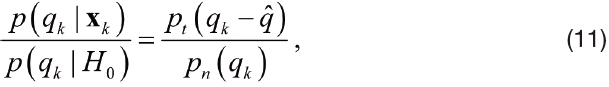
As the target state is assumed as the Markov process, the result of each stage depends only on the results of the previous stage. The maximum possible value of the scoring function for collision threat is obtained by the inclusion of a sequence of intermediate functions that represent the maximum partial sum of the previous scoring functions. Based on the posterior odds formulation, the scoring function,
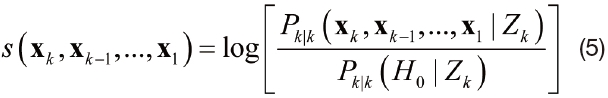
where (x

In every successive DP processing stage both the maximizing value of x
where
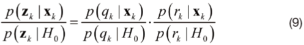
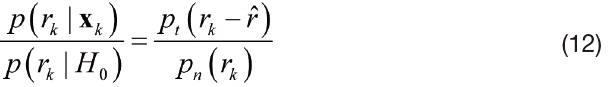
It is usually quite reasonable to assume that given the true state x, the target amplitude is independent of the rate of the target expansion. The target amplitude of the pointlike target depends on the noise sources that are created by the change of weather such as clouds or lighting conditions. On the other hand, the rate of expansion is a function of the relative distance between the target and own aircraft [5]. With this assumption, the second term on the right-hand side implies that
where
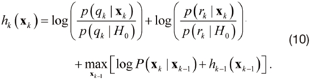
In the recursive update equation, the function
2.4 Implementation of Dynamic Programming
In order to detect target expansion, a sub-window around each pixel was explored. The sub-image that corresponds to the window is convolved with a smoothing mask. This mask performs low-pass filtering for the output considered as the measure of target strength. This measurement is obtained in terms of the increase of the target strength and it is tracked over a number of stages. The mean rate of expansion was estimated by applying least squares to the target strength.
The probability density functions of the observations are based on the prior knowledge of amplitude and noise characteristics of potential collision threats. These distributions are also adaptively determined from the observation sequence. As the given measurement noise is additive, the likelihood ratio becomes,
where

and

are the anticipated target characteristics. In order to model the two output characteristics, a standard Gaussian distribution is developed, whereas the parameters of the distribution are empirically chosen from the data. Other various non-Gaussian distributions can be used to more accurately reflect on the highly nonlinear characteristics of observations [3].
The transition cost function accounts for the probability of target maneuvers and the noise properties of optical sensors. The transition cost is derived from both a priori models for target maneuvers and the models for state resolution cell quantization and errors in image processing steps. The transition probability is a function of the absolute difference between the expected and actual state at state

As the innovation of the target state is assumed to be independent in time and dimension, the transition costs are separable into the product of transition probabilities of each dimension. These transition probabilities are to be computed from the difference of the Gaussian error functions that are given by,
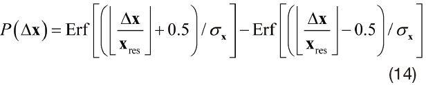
where Δx is the difference between the current state and the predicted state, Erf is the Gaussian error function,

is the floor function, σx is the standard deviation of the target innovations in terms of resolution cells and xres is the resolution of the quantized states.
A DP-based TBD method is based on the proposed track scoring function which is implemented and evaluated by using a synthetic image sequence. In order to carry out the trial our simulation study requires, the image sequence with 100 frames and a frame size of 32 by 32 pixels at 10 frames per second. This is synthetically generated. The image sequence contains the simulation of a moving target that moves through a structured background. A motion effect is caused by jitter and an aperture effect from the optics is also added onto the overall sensor model. In this image sequence, a single artificial target with relatively bright amplitude appears at the 20th frame and it flies from the center to the lower right. The target gradually expanded from the point to the shape of a plus sign that is defined by the image intensity at each pixel position in order to emphasize the target detection capabilities for objects on a collision course.
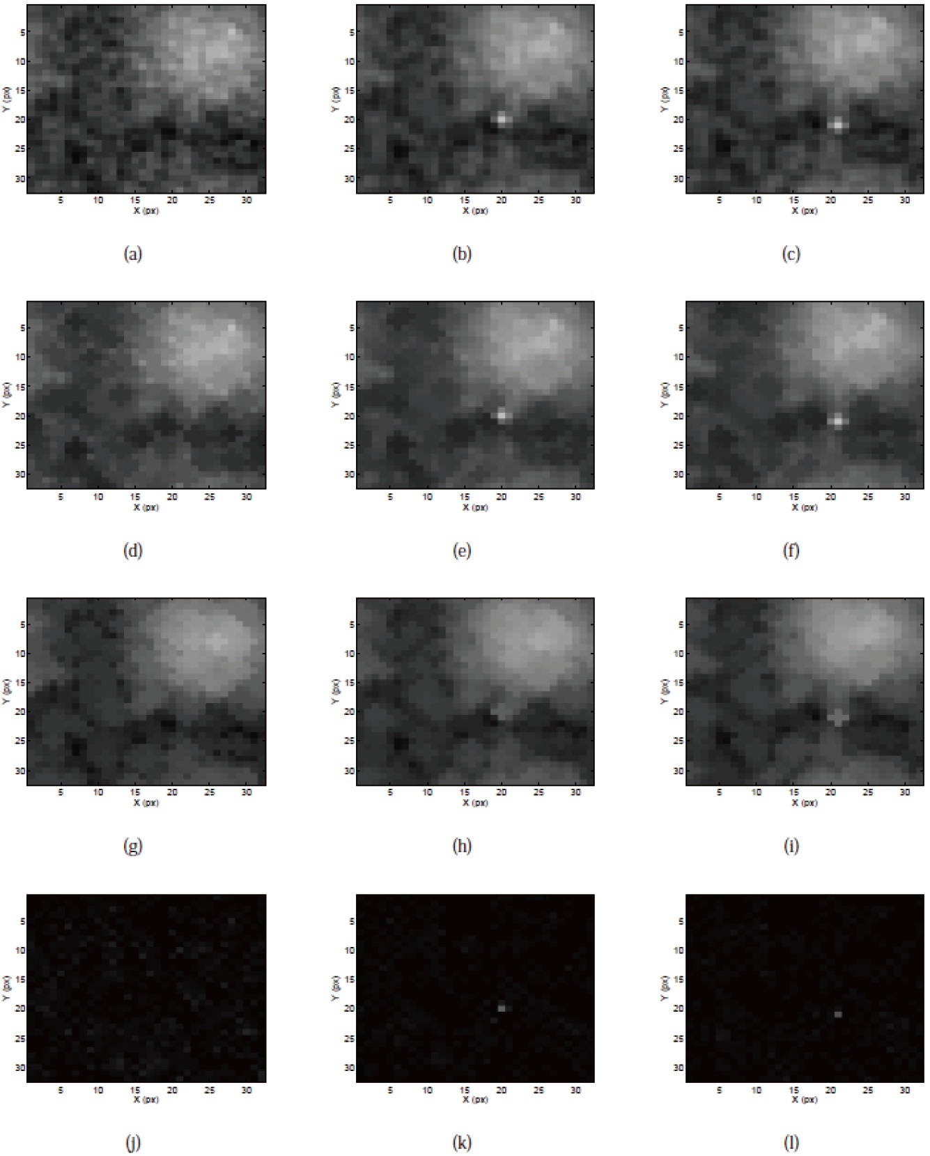
The results of gray-scale morphological filtering are
shown in Fig. 2 for the three chosen images. Figures 2.(a)- (c) shows the raw input images from the image sequence. Figures 2.(d)-(f ) show the results of closing and this tends to preserve small brighter than the background. Figures 2.(g)- (i) show the results of an opening and this tends to remove the bright regions that are small in size. Overall image processing results are shown in Figs. 2.(j)-(l). They confirm that the CMO morphological filtering has removed large clutters such as clouds in the background in order to extract point-like targets.
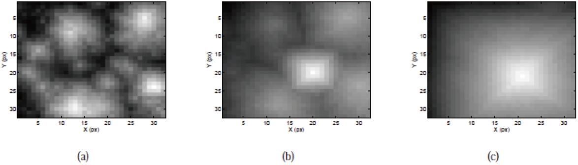
The simulation parameters are given in Table 1. Figure 3 shows the results of the DP algorithm. The displayed intensity value has been scaled to reflect the track scoring for each spatial resolution cell in the chosen velocity plane. The target appears as a bright area which moves near the center of the image in Figs. 3.(b)-(c). The increased signal strength reflects the consistent integration procedure by the DP-based TBD
method. This increase in both the size and amplitude of the target is considered in the track scoring function.
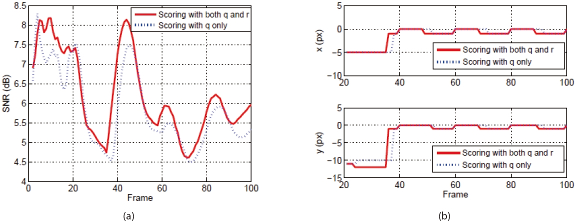
Figure 4 shows a comparison of the track scoring functions by taking into account the two different observation sets. The
[Table 1.] Summary of the simulation parameters
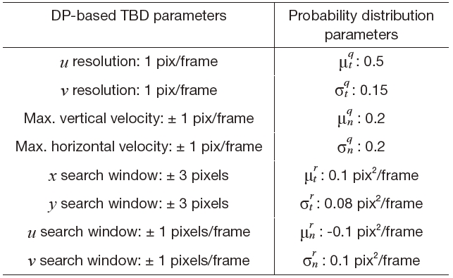
Summary of the simulation parameters
first observation set provides both
In this paper, a track scoring function of DP-based TBD method is proposed to take account of the two distinguishable properties of airborne targets on a near-collision course. The findings from the numerical results indicate that the signalto- ratio with the modified track scoring function is slightly improved compared to the previous one. Further work is being undertaken and it includes the implementation of the DP-based TBD method applied for airborne target detection.