Acknowledgement of the threat to planet Earth from the impact of an asteroid or comet has led to increased interest in studying asteroid intercept and rendezvous missions. In addition to responding to a threatening asteroid, scientific missions to asteroids and other small bodies are of interest. NASA’s Deep Space 1 and Deep Impact missions, and JAXA’s Hayabusa mission are examples of flyby, intercept/impact, and rendezvous, respectively. The differing mission requirements and spacecraft capabilities will require continued study on terminal-phase guidance laws.

This paper will review a number of different feedback guidance laws, starting with simple laws to enable intercept, then going through more sophisticated laws, including laws with specified terminal conditions, and optimal feedback guidance laws. Simulation results are shown, proving the practical effectiveness of such feedback guidance laws.

Proportional navigation (PN) guidance is one of the earliest known feedback guidance laws. Zarchan [1] describes PN guidance, as well as a method of augmenting it when acceleration characteristics of the target are known or can be assumed. These feedback guidance laws can be implemented with on-off thrusters using a simple Schmitt trigger or other pulse-modulation devices as described in Wie [2]. Zarchan [1] also describes predictive guidance for targets whose primary acceleration is due to a gravitational field. This is based on Lambert’s theorem. Linearized predictive guidance is possible, based on the state-error transition matrix described by Vallado [3].

Gil-Fernandez et al. [4, 5] describe various terminal-phase guidance laws of a kinetic impactor as applied to the European Space Agency’s Don Quijote mission (now cancelled). This work was continued in more detail by Hawkins et al. [6].

Much work has been done on the problem of commanding intercept at a specified impact angle. Some of the earliest work led to guidance laws with strict limits on initial conditions [7]. Since then, a number of different laws with different advantages have been proposed. Various guidance laws exist that do not require the time-to-go [8] that allow for significant target maneuvers [9] and that can be used during hypersonic flight [10]. Linear-quadratic control laws have been derived in [11], and guidance laws based on classical proportional navigation are described in [12]. Guidance laws have been derived to follow a circular path to the target [13] and to establish the desired end-of-mission geometry early on [14]. Hawkins and Wie [15] investigated modified PN guidance laws for asteroid intercept with terminal velocity directional constraints.

Bryson and Ho [15] discussed optimal feedback control laws for a simple rendezvous problem, considering both free-terminal velocity and constrained-terminal velocity. They also discussed the relationship between optimal feedback control and proportional navigation guidance. Battin [16] also discussed an optimal terminal-state vector control for the orbit control problem, directly compensating for the known disturbing gravitational acceleration. D’Souza [17] further examined an optimal control algorithm in a uniform gravitational field, and developed a computational method to determine the optimal time-to-go.

Guo et al. [18] found three different optimal control laws for certain constraints on terminal conditions. All three laws require the terminal position to be specified, while the terminal velocity can be fully specified, free, or constrained along a particular direction. Hawkins et al. [19] compared these guidance laws with PN-based guidance laws.

Ebrahimi et al. [20] proposed a robust optimal sliding mode guidance law for an exoatmospheric interceptor, using fixed-interval propulsive maneuvers. In this paper, gravity was considered to be an explicit function of time. One major contribution of Ebrahimi et al. was the new concept of the zero-effort-velocity (ZEV) error, analogous to the well-known zero-effort-miss (ZEM) distance. The ZEV is the velocity error at the end of the mission if no further control accelerations are imparted. Furfaro et al. [21] later employed the ZEM/ZEV concept to construct two classes of non-linear guidance algorithms for a lunar precision landing mission.

Guo et al. [22, 23] showed that in a uniform gravitational field, the ZEM/ZEV logic is basically a generalized form of various well-known optimal feedback guidance solutions such as intercept or rendezvous, terminal guidance, and planetary landing. A Mars landing example, originally described by Acikmese and Ploen [24] is investigated in [23, 24]. In some cases ZEM/ZEV guidance can be improved by introducing a number of waypoints. Details are given in [23, 24] on how to practically compute such waypoints in real time. Finally, the ZEM/ZEV concept was also generalized to other feedback guidance problems in [23, 24].

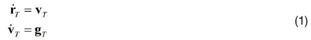
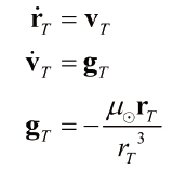
The target asteroid can be modeled as a point mass in a standard heliocentric Keplerian orbit, as follows:

where r_T and v_T are the position and velocity vectors of the target and g_T is the gravitational acceleration due to the sun, expressed as

where μ_⊙ is the solar gravitational parameter. Similarly, the motion of the spacecraft is described by

where r_S and v_S are the position and velocity vectors of the spacecraft, g_S is again the gravitational acceleration acting on the spacecraft due to the sun, and a is the control acceleration provided by the spacecraft thrusters. In this paper, a boldfaced symbol indicate a column matrix of a physical vector expressed in a chosen inertial reference frame.

In general, we have g = g(r, t). For some guidance problems the gravitational acceleration can be considered constant or negligible, but in general, the gravitational acceleration must be considered a nonlinear function of position. There are some other disturbing accelerations that act on the spacecraft, such as solar radiation pressure and the gravitational acceleration due to the asteroid. However, intercept and rendezvous missions to small asteroids can neglect these.

The relative position of the spacecraft with respect to the target asteroid is then described by

The equation of motion of the spacecraft with respect to the target becomes

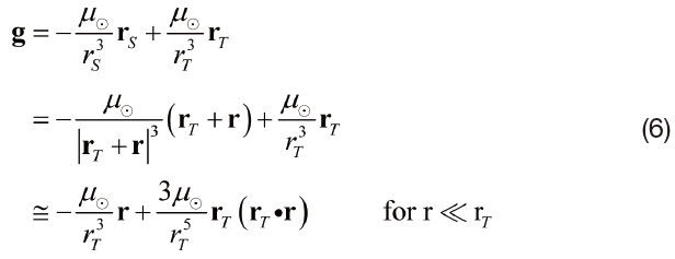
where g represents the sum of apparent gravitational accelerations on the target, as follows:

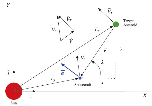
From Figure 1, it can be seen that

where λ is the line-of-sight (LOS) angle and (x, y) are the components of the relative position vector along the inertial (X, Y) coordinates. Differentiating this with respect to time gives

where

is the LOS rate and

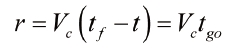
The rate of change of the distance between the target and the spacecraft is the closing velocity, found by differentiating r with respect to time as

3.1.1 Classical Proportional Navigation (PN) Guidance

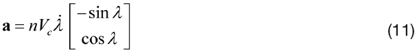
The first guidance law considered in this paper is the so-called proportional navigation (PN) guidance. The PN guidance attempts to drive the LOS rate to zero by applying accelerations perpendicular to the LOS direction. The PN guidance law is expressed as

where a is the acceleration command and n is the effective navigation ratio, a designer-tunable parameter [1]. The navigation ratio is typically chosen between 3 and 5. The optimal value, which will be derived and discussed in a later section, is 3. Larger values are chosen to provide more robustness against disturbances and errors. This can be seen by inspecting Eq. (10). Inaccurate estimates of the closing velocity or the LOS rate are equivalent to changing the navigation ratio and using accurate closing velocity and LOS rate information. Large navigation ratios will command unnecessarily large accelerations, while small navigation ratios risk commanding too little acceleration and missing the target. Thus a larger navigation ratio ensures that measurement errors will not make the accelerations too small to achieve impact.

Because the acceleration commands are chosen to be perpendicular to the LOS, the PN guidance law gives a scalar value. The PN guidance acceleration command is then expressed in the inertial reference frame as

The PN guidance law for steering an interceptor is also called constant-bearing guidance, because it steers the interceptor in such a way that the LOS does not rotate. An interceptor using PN guidance, on a perfect collision course, will maintain a constant bearing (i.e.,

is zero). When the interceptor is not on a collision course, the trajectory is not truly constant-bearing for n < ∞. As the effective navigation ratio becomes very large, the LOS rate approaches zero faster, at the expense of larger commanded acceleration.

The PN guidance law does not require the target or interceptor velocities to be constant, nor does it require the external accelerations to be zero. For small deviations from constant velocity and small external accelerations, the PN guidance law will still achieve intercept in a feedback fashion. For the asteroid intercept scenario, the velocities are approximately constant, and the external acceleration is due almost entirely to the sun, and can be accounted for as described below.

3.1.2 Augmented PN Guidance

The basic PN guidance law can overcome target accelerations in a feedback fashion. As can be seen from the equations for LOS rate and closing velocity V_c, Eqs. (8) and (9), the PN guidance law uses only the position and velocity of the target, and is unable to take into account target accelerations (if they exist). A guidance law which incorporates terms to account for the target’s acceleration should be able to perform better than the basic PN guidance law. Since the primary target accelerations are from the sun’s gravity, the target’s future accelerations are known. An augmented proportional navigation guidance (APNG) law will now be discussed. As with PNG, an easily tractable derivation will be given first, and optimality will be considered in a later section.

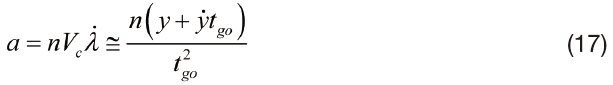
From Figure 1, with a small-angle approximation, we have

where y is the spacecraft-target distance perpendicular to the reference line (X-axis). Define the mission time-to-go as

For a successful intercept mission, the separation at the end of the flight is zero, or r(t_f) = 0. Integrating Eq. (9) gives

Substituting Eq. (14) into Eq. (12) gives

Differentiating this expression gives

Using this expression in the PNG law gives

For PN guidance, we define the Zero-Effort-Miss (ZEM) distance as the separation between the target and the interceptor at the end of the flight, absent any further control accelerations. With no accelerations, the interceptor and target will continue on straight-line trajectories. The components of the ZEM can thus be given as

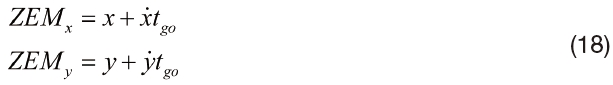
The ZEM is a simplified prediction of future target-interceptor separation. PN guidance commands are always applied perpendicular to the LOS, therefore only the component of the ZEM that is perpendicular to the LOS can be accounted for in the augmented guidance law. From trigonometry, this component is

The PNG law, Eq. (10), is now rewritten as

A constant acceleration can be added to the ZEM term. The linearized ZEM equation is now

where a_T is the apparent target acceleration as seen by the spacecraft. Substituting this into Eq. (20), and using Eq. (17), gives

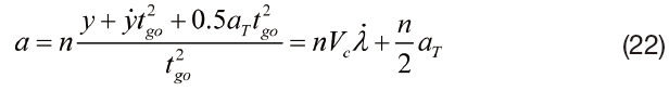
In general, for the asteroid terminal intercept scenario, the sun’s gravity is the primary disturbing force that needs to be accounted for. The above augmented proportional navigation guidance law can easily incorporate the effect of gravity. The APNG law issues commands perpendicular to the LOS, and from the spacecraft’s point of view. Thus the acceleration term needed is the relative solar acceleration perpendicular to the LOS. To begin, the components of the gravity term for the target and the spacecraft are

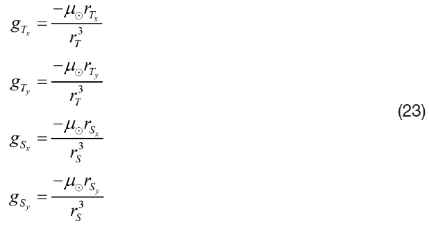
The components perpendicular to the LOS are

The target’s apparent acceleration perpendicular to the LOS, as seen by the spacecraft, is

Substituting this equation into the APNG law, Eq. (22), gives

In the inertial reference frame, the APNG law is expressed as

As with PNG, the optimal navigation ratio for APNG is 3, to be discussed in a later section.

3.1.3 Pulsed Guidance

For a simple intercept problem, the terminal velocity is not specified, and is assumed to be the closing velocity for PNG and APNG. The PNG and APNG laws assume that continuously variable thrust is available. For thrusters with no throttling ability, a different approach to guidance laws is needed. Two approaches to formulating guidance laws for fixed-thrust-level (on-off) guidance laws are PN-based guidance laws and predictive guidance laws.

The PNG law continuously generates acceleration commands to achieve intercept. Due to its feedback nature, PNG will continue to generate guidance commands until intercept is achieved. A special case of PNG occurs when the interceptor is on a direct collision course. When this is true, the guidance commands will be zero. When using PNG logic, then, an acceleration command of zero means that the interceptor is instantaneously on a direct collision course. This fact can be exploited to use PNG logic for constant-thrust engines.

Pulsed PNG (PPNG) logic computes the required acceleration commands from PNG, but applies them in continuous-thrust pulses. PPNG will “overshoot” the amount of correction specified by PNG, until the PNG command is zero. At that point, the interceptor is instantaneously on a collision course, and the engines are turned off. If there were no external accelerations or disturbances, the interceptor would continue on an interception course. Because of the acceleration due to the sun, this will not be the case, and a further engine firing will be required later as the interceptor “drifts” further and further from the straight-line collision path.

Two approaches to determining when to fire engines are threshold methods and timed methods. Both methods will be described, as well as advantages and disadvantages associated with each approach.

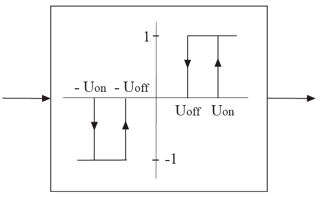
The threshold method can employ the so-called Schmitt trigger or other pulse-modulation schemes [2]. Using a Schmitt trigger, acceleration commands are calculated by the PN guidance law as before. The trigger commands the divert thrusters to turn on once the commanded acceleration exceeds a certain magnitude, chosen by the designer, and off when the commanded acceleration reaches a designer-chosen cutoff. With traditional PN guidance the LOS rate must reach zero for a successful intercept. Therefore the second cutoff is typically selected as zero. The Schmitt trigger control logic for pulsed proportional navigation guidance (PPNG) is shown in Figure 2. The Schmitt trigger can also be used for augmented PN guidance, giving an augmented pulsed proportional navigation guidance (APPNG).

The timed method is similar to the threshold method in that the PNG commands are still calculated, and applied with constant thrust. As the name suggests, the difference is that the timed method uses predetermined firing times to turn on the thrusters. The designer must choose the firing schedule. Typically at least three firings are required. An early firing, near or at the beginning of the terminal mission phase, is used to overcome most of the orbit injection errors. The final firing comes shortly before impact, with enough lead time to allow the thrust command to complete (e.g. the commanded acceleration reaches zero), but close enough to impact that only minimal further errors accumulate. Additional intermediate firings provide robustness. As with the Schmitt trigger, the timed method turns off thrusters when the commanded thrust level is zero.

The advantage of these methods is the ability to use constant-thrust on-off engines. The Schmitt trigger has the same feedback advantages as PNG, in that it will issue commands when the spacecraft is not on an intercept course. A disadvantage of the Schmitt trigger is that the designer must select the magnitude to turn on the thrusters. Too small a magnitude risks excessive on-off cycles (chatter) for the engines, while too large a magnitude risks missing the target by failing to issue commands at all. An advantage of the timed method is that the total number of on-off cycles is known in advance and can be kept small. A disadvantage is that the timed method might not issue commands even when the calculated PNG commands are large.

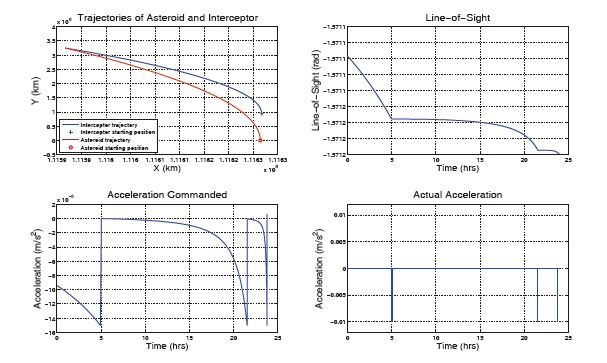
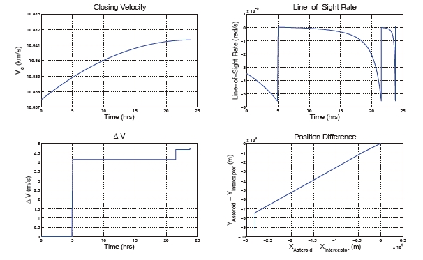
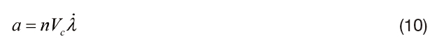
The pulsed PN guidance law described in this section was applied to an asteroid intercept problem in [6]. A fictitious 300-m asteroid is assumed to be in a circular orbit with a radius of one astronomical unit. An interceptor with closing velocity of 10.4 km is displaced 350 kilometers out radially. It is displaced 24 hours travel time ahead of the target in the tangential direction. In the absence of guidance commands, the assumed initial conditions will result in a miss distance of 88.29 km. A 1000-kg interceptor with two 10-N divert thrusters is assumed. Simulation results summarized in Figures 3 and 4 indicate that the pulsed PN guidance system performs well. More detailed discussions of this asteroid intercept example problem can be found in [6].

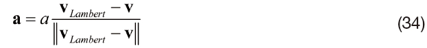
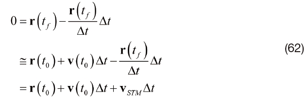
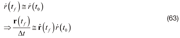
A different class of guidance laws, which also use on-off pulses, are the predictive guidance schemes. Two types of predictive guidance laws are Lambert guidance and time-varying state transition matrix (STM) guidance. Both types of predictive feedback guidance laws will command a required velocity, v_req. Subtracting the current velocity v from this gives the velocity to be gained, or Δv. The simplest way to generate acceleration commands is to align the thrust vector with the Δv vector. When the desired velocity is achieved, Δv is zero

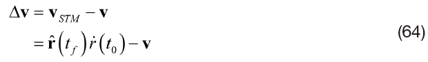
and the engine is cut off. The velocity to be gained is

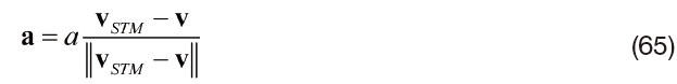
For a given acceleration magnitude a, the direction of the thrust acceleration should be aligned with the velocity-to-be-gained vector; that is, we have

3.2.1 Lambert Guidance

The well-known Lambert’s theorem, a two-point boundary value problem (TPBVP), states that “the orbital transfer time depends only upon the semi-major axis, the sum of the distances of the initial and final points of the arc from the center of force, and the length of the chord joining these points” [17]. Mathematically, Lambert’ theorem is expressed as

where t₂ ？ t₁ is the time of flight, c = ||r₂ ？ r₁||, and

is the semi-major axis of the transfer orbit. The solution of Lambert’s problem determines the required transfer orbit from position r₁ to r₂ in time t₂ ？ t₁. The current position of the spacecraft is known, and the desired time-of-flight can be calculated. Recall Eq. (14)

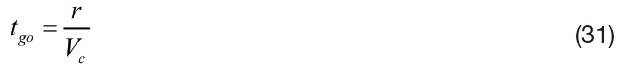
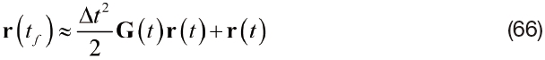
The time-to-go is thus calculated as

The position of the target at the end of the flight time can be estimated by numerically integrating the target’s current

position and velocity over the time-to-go. Many different Lambert solvers have been developed that take the position vectors r₁ and r₂, and the time of flight as inputs, and give parameters of the transfer orbit as output, including v₁ and v₂, the velocity of the transfer orbit at the initial and final times. The initial velocity is the required velocity from the Lambert solver routine, v_Lambert. The required velocity is thus

Comparing with Eq. (28) gives

The acceleration command is explicitly given as

The Lambert guidance routine requires a firing schedule to decide when to perform thrusting maneuvers. In principle, one Lambert guidance engine burn should suffice to achieve impact. In practice, multiple engine burns should be used to account for errors in calculating and applying velocity corrections. Similar to PPNG with timed firings, a minimum of three burns is often used.

3.2.2 Time-varying State Transition Matrix (STM)

Impulsive guidance laws can also be formulated using the state transition matrix concept. In this approach, the target asteroid’s orbit is considered to be a known, or reference, orbit. The interceptor’s orbit is considered to be a perturbation from this reference orbit. The goal is then to issue guidance commands that will drive the position perturbation to zero.

Recall the dynamical equations of motion for the target asteroid

In this section, the standard notation of orbital perturbation theory will be followed. This notation differs from that used in the rest of the paper, but is used because it is more germane to the problem. The target state is the reference state, x*. The spacecraft state, x, is the target state plus some deviation δx, defined as

where

When components of the spacecraft state are needed, they will be given in orthogonal directions denoted with 1 and 2. The subscript S will be dropped for notational simplicity, but it is important to note that these are components of the spacecraft state, and not the spacecraft’s relative state. The spacecraft state vector x is then defined as

Consider the target asteroid trajectory to be a known, or reference, trajectory. The equations of motion for the spacecraft trajectory are, in general, a function of both state and time as described by

More explicitly, we have

Substituting Eq. (35) into Eq. (38) gives

Equation (40) is nonlinear, so it can be expanded in a Taylor series about x*, as follows:

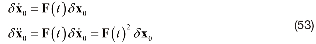
Substituting the time derivative of Eq. (35) into Eq. (41) gives

Recall that the target orbit is considered to be the known reference orbit. As such, the position and velocity are known for any given time. The function f and the state x can therefore be considered functions of time alone. The equation of motion for the state deviation is then simply expressed as

where F is the partial derivative term in Eq. (42), which is the Jacobian of the function f evaluated at x* defined as

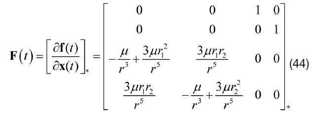
where

is replaced with μ for notational simplicity. Recall that the acceleration due to the sun’s gravity, Eq. (2), is

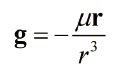
The Jacobian of the gravitational force vector is often called the gravity-gradient matrix defined as follows:

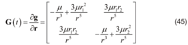
Observe that this corresponds to the bottom-left submatrix of F, which can be written as a block matrix

where I and 0 are the identity matrix and the zero matrix of conformal (in this case 2×2) size.

The general solution to Eq. (43) above can be expressed as

where δx₀ = δx(t₀). Differentiating this gives

Substituting Eq. (48) into Eq. (43), and using Eq. (47), we have

This must be true for any δx₀, thus

with initial conditions given by

Equation (50) can be numerically integrated, starting with the initial conditions given in Eq. (51), to find the current estimate of the state transition matrix. However, for use in generating a guidance law for asteroid intercept, it is desirable to avoid numerical integration. As will be discussed in a later section, if a numerical integration is to be performed, it is better to simply integrate the equations of motion directly. It is desirable to have an analytical expression of Φ for use in guidance laws.

Consider the expression for the state error. Expanding this into a Taylor series gives

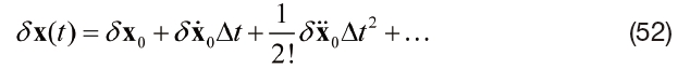
Recalling Eq. (43), and taking its derivatives, gives

Comparing Eqs. (47) and (52) gives

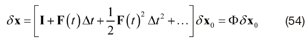
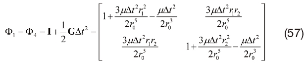
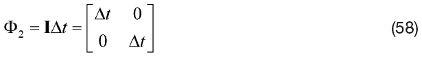
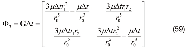
Evaluating the expression in brackets gives the state-error transition matrix as

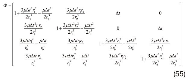
This state-error transition matrix can be partitioned as

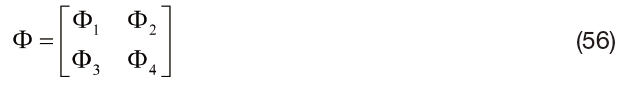
where

The simplest form of intercept guidance using the state-error transition matrix uses only the position information to generate a Δv command. The first-order approximation for the final miss vector, absent any further acceleration commands, is found as

The second term on the right-hand side is negligible for small changes in closing velocity, giving

Consider driving the final relative position to zero. For linearized dynamics, there are no external accelerations, so we have

where v_STM is seen to be the velocity to be gained to ensure impact.

For small changes in relative velocity, we have

The velocity change to be imparted becomes

The acceleration command vector is given, similar to Lambert guidance, as

Using the gravity gradient matrix from Eq. (45), we can show that

3.2.2.1 Predictive Impulsive Guidance

For practical implementation, we adopt the following definitions

Substituting these into the guidance law in Eq. (64) gives the predictive impulsive guidance law

3.2.2.2 Kinematic Impulsive Guidance

In terms of the line-of-sight angle, we have

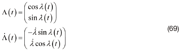
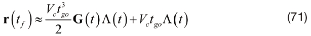
The relative position can also be approximated as

and we obtain

The relative velocity can be approximated as a component along the LOS and a component perpendicular to the LOS, described as

Substituting Eq. (72) into Eq. (68) results in the kinematic impulsive guidance law of the form

For some applications it is desirable to specify terminal conditions on the interceptor. For intercept, the terminal position is by definition zero. The terminal velocity, though, may have direction or magnitude requirements, depending on the mission. Optimal feedback guidance laws can be used to achieve intercept, with the option of specifying the final velocity.

Three different optimal feedback guidance laws are considered for asteroid intercept and rendezvous missions. The various forms of proportional navigation and predictive guidance laws compute an estimated mission time-to-go based on relative position and velocity. This computed time-to-go is used as an input for the predictive laws, and is available as an output of the proportional navigation laws. In contrast, the optimal feedback guidance laws use a specified time-to-go as a mission parameter, and compute the acceleration commands needed to achieve intercept at this pre-determined time.

When the final impact velocity vector (both impact velocity and impact angle) is specified, the terminal velocity is constrained. This leads to the constrained-terminal-velocity guidance (CTVG) law. If the final velocity is free, the free-terminal-velocity guidance (FTVG) law results, as discussed in [18, 19]. When only the approach angle is commanded, the velocity vector component along the desired final direction is free, while the perpendicular components are constrained to be zero. A combination of FTVG along the impact direction and CTVG along the perpendicular directions allows pointing of the final velocity vector, referred to as interceptangle- control guidance (IACG).

3.3.1 Constrained-Terminal-Velocity Guidance (CTVG)

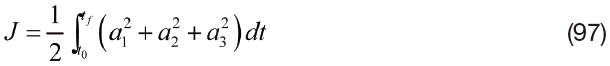
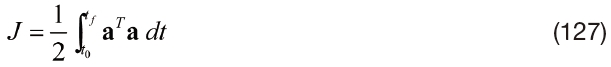
Consider an optimal control problem for minimizing the integral of the acceleration squared, formulated as

subject to

and

with the following boundary conditions

The Hamiltonian function is given by

where p_r and p_v are co-state vectors associated with the position and velocity vectors, respectively. In general, for a terminal-phase guidance problem gravity is a function of position and time, g = g(r, t). Using such a function will not allow a simple closed-form solution to the optimal control problem. For the class of terminal guidance problems considered in this paper, the gravitational acceleration is approximately constant for the duration of the terminal phase. Therefore, a constant gravitational acceleration is assumed to permit an analytical closed-form solution. The co-state equations and control equation imply that

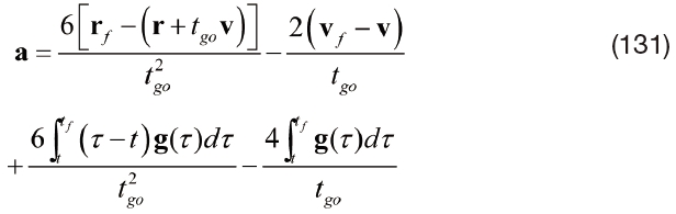
For fixed terminal conditions, the co-states at t_f are nonzero. Define t_go = t_f ？ t as the time-to-go before arrival at the terminal state, and let p_r(t_f) and p_v(t_f) describe the value of p_r and p_v at t_f, respectively. Integrating the co-state equations yields

Substituting Eq. (81) into Eq. (79) yields the optimal control solution as

The states can thus be expressed as

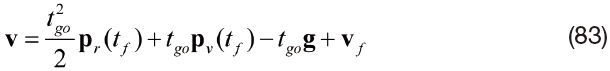
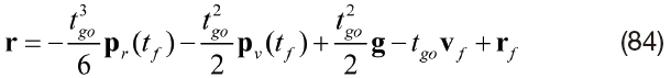
Combining Eq. (83) and Eq. (84) leads to

Finally, the optimal feedback control law with specified r_f, v_f, and t_go, the CTVG law, is obtained as

or

Figure 3 shows a family of asteroid intercept trajectories using CTVG. In all cases the spacecraft starts 2 km from the target, with initial velocity of [50,0,0] m/s.

3.3.2 Free-Terminal-Velocity Guidance (FTVG)

For the case when the terminal velocity is free, the boundary conditions for unconstrained final velocity give p_v(t_f) = 0, thus Eq. (81) p_v becomes

The acceleration command is then given as

Accordingly we have

Solving the above equations results in

The terminal velocity can be expressed in terms of time-to-go and system states after substituting Eq. (93) into Eq. (91), as

which is a function of time with given initial position and velocity vectors.

Substituting Eq. (93) into Eq. (90), the FTVG law is obtained as follows

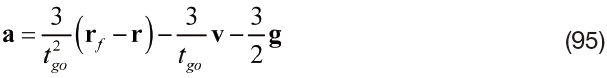
Figure 4 shows a family of asteroid intercept trajectories using FTVG. The initial conditions and final position are fixed, but the total flight time is varied.

3.3.3 Intercept-Angle-Control Guidance (IACG)

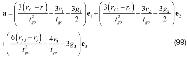
Both CTVG and FTVG command the final position. The terminal velocity vector can be commanded, as in CTVG, or free as in FTVG. Consider an orthogonal coordinate system with the first component e₁ in the direction of the desired terminal velocity, and the other two components (e₂, e₃) perpendicular to this direction. The acceleration vector can be expressed as

The performance index then becomes simply

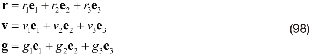
The position, velocity, and gravity vectors can also be expressed as

In order to achieve impact along the e₁-direction, it is required that v₁ is free, and v₂ and v₃ are both zero. The IACG algorithm combines the CTVG and FTVG algorithms as follows:

This algorithm can also be expressed in terms of vectors r, r_f, v, and g as

It is important to note that the IACG guidance law does not impose a unique direction on the final velocity. Ultimately, the velocity is only constrained to be parallel to the specified direction. The final velocity direction will depend on the initial conditions. If the spacecraft is initially moving toward the target in the e₁ direction, that is, (r_f1 ？ r₁)v₁ > 0, then the intercept will be in the specified direction. Otherwise, when (r_f1 ？ r₁)v₁ ≤ 0, the spacecraft will intercept opposite the specified direction. Figure 5 shows a family of asteroid intercept trajectories using IACG. The spacecraft’s initial speed is 100 m/s in all cases, with different initial directions. Intercept is always directed to occur along λ_f = 0.

3.3.4 Relationship between PNG and Optimal Feedback Guidance

As mentioned in the section on PNG, the optimal value for the navigation constant is 3 [1]. To show this, first consider a two-dimensional problem with

where λ is the LOS angle as before. Defining R = |r_f ？ r| as the distance from the spacecraft to the target along the LOS. The closing velocity and time-to-go are given by

The optimal FTVG algorithm thus becomes

This is the augmented PNG logic, with an effective navigation ratio of 3.

Controlling the direction of the final velocity is equivalent to controlling the final impact angle, but not the velocity. Since the PNG laws only command control perpendicular to the LOS, the velocity along the LOS is free. For the case with small LOS angles, it can be shown that IACG becomes PNG with impact angle control

where λ_f is the desired final impact angle.

3.3.5 Calculation of Time-To-Go

The basic PNG laws do not specify the time-to-go, and can estimate it based on current conditions. In contrast, the optimal feedback guidance laws are derived for a fixed flight time. The time-to-go appears in the acceleration commands. For some missions it may be desirable to specify the mission flight time. However, for asteroid intercept it is often not necessary to achieve impact or rendezvous at a particular time, and a difference of a few seconds or minutes is not significant to the overall mission.

Consider, for example, an interceptor that is already on a collision course with the target. Proportional navigation guidance will not issue any commands, and intercept will occur based on the interceptor’s velocity relative to the target. If one of the optimal feedback guidance laws is used with a different time-to-go, intercept will still occur, but the spacecraft will spend unnecessary fuel either speeding up or slowing down the spacecraft along the LOS direction. It is natural to ask, then, if there is an optimal choice for time-to-go.

For both the CTVG and FTVG laws, under certain conditions a local minimum for the performance index with respect to mission time is possible [18, 19]. This condition will be derived next. It is important to note that the optimal feedback control laws minimize the integral of acceleration squared, and not ΔV or fuel use.

3.3.5.1 CTVG

As was the case when deriving the CTVG law, the gravitational acceleration is assumed to be constant to permit a closed-form solution. The transversality condition is given by

The Hamiltonian function of the form

becomes

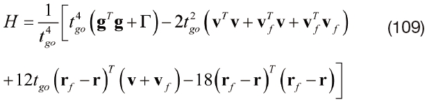
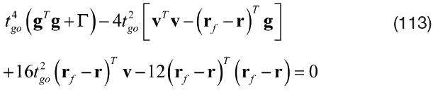
Equation (107) then gives

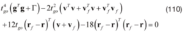
which can be solved for the time-to-go. Note that the first term in the above equation contains the fourth power of the time-to-go, and the unknown parameter Γ. This first term is also the only term where the gravitational acceleration appears. By assuming that g is negligible, and setting Γ to zero, Eq. (110) simplifies to

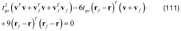
The time-to-go can be calculated as follows:

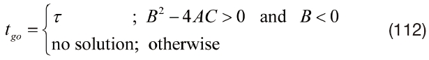
where

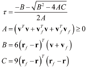
and τ is the smaller positive solution of Eq. (111), leading to a local minimum of J*. The larger solution corresponds to a local maximum of J*. J* decreases monotonically with respect to t_go for values beyond the larger solution. When there is no solution, the partial derivative of J* is always negative, thus increasing t_go leads to decreasing J*.

3.3.5.2 FTVG

A similar procedure can be used to compute the time-to-go for the FTVG law. The condition corresponding to Eq. (110) is

When g = 0 and Γ = 0, this becomes

Let θ be the angle between the vectors v and (r_f ？ r). The solution of equation (114) is obtained as

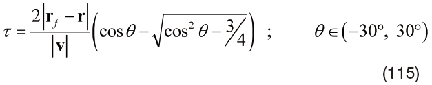
There is a finite solution only when θ lies in the range (？30°, 30°).

There is no general way to derive an optimal time-to-go for IACG. Recall that IACG consists of FTVG along the final impact velocity direction, and CTVG perpendicular to this. Typically, then, there will be two different optimal times, and the true local minimum will be dependent on the particular mission geometry.

In the preceding section, the optimal feedback guidance laws were discussed assuming a uniform gravitational field (g = constant). If g is an explicit function of time, it is also possible to derive the optimal CTVG and FTVG algorithms.

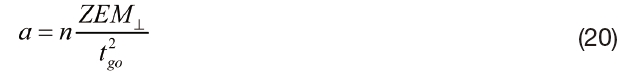
Let the zero-effort-miss (ZEM) be the position offset at the end of the mission if no more acceleration is applied. Also let the zero-effort-velocity (ZEV) be the end-of-mission velocity offset with no acceleration applied. The dynamic equations of motion with no control acceleration are

These equations can be integrated to find the ZEV and ZEM as

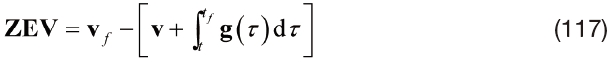
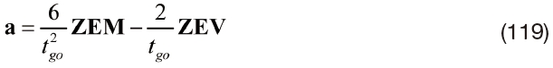
With the ZEM and ZEV defined as above, the ZEM/ZEV version of the CTVG law is expressed as

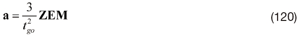
The FTVG law is expressed as

As was the case for the optimal feedback laws, the ZEM/ZEV laws are optimal for a specified flight time. When a particular flight time is needed as a mission requirement, ZEM/ZEV laws can be applied using that flight time. If the exact flight time is not important, some additional analysis can be applied to find the optimal flight time. The optimal flight times found above for CTVG and FTVG, for example, can be used as a starting point for the optimal flight time.

3.4.1 Estimation the ZEM and ZEV

For the case when gravity is not constant, the ZEM and ZEV must be estimated. There are three basic options, of varying complexity. The most complex option is simple numerical integration of the equations of motion. This method is computationally intensive, but will result in the most accurate estimates of ZEM and ZEV.

The second option employs the time-varying STM. Recall that the ZEM is the difference between the desired final position and the final position in the absence of corrective maneuvers. For the asteroid intercept/rendezvous problem, this can be expressed as

where r(t_f) is the predicted spacecraft position at t = t_f and r_f is the desired final position. Then the ZEM estimate using the time-varying STM becomes

Similarly, the ZEV can be estimated as

Finally, for cases when the gravitational force is not significant, the ZEM and ZEV can be estimated by direct linearization of the relative states. Ignoring any external accelerations, we can estimate the ZEV as the current relative velocity and the ZEM as the current relative position plus the relative velocity times time-to-go, described as

3.4.2 Optimal Feedback Guidance Algorithms for a Special Case of g = g(t)

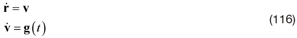
The gravitational acceleration is, in general, a function of position, which will not lead to an analytical solution of the optimal control problem. However, if the gravitational acceleration is assumed to be an explicit function of only time, then the analytical optimal solution can be found.

For a mission from time t₀ to t_f, the optimal control acceleration needs to be determined by minimizing the standard performance index of the form

subject to Eq. (116) and the following given boundary conditions:

The Hamiltonian function for this problem is then defined as

where p_r and p_v are the co-state vectors associated with the position and velocity vectors, respectively.

The co-state equations provide the optimal control solution expressed as a linear combination of the terminal values of the co-state vectors. Defining the time-to-go, t_go, as t_go = t_f ？ t. The optimal acceleration at any time t is expressed as

By substituting the above expression into the dynamic equations to solve for p_r(t_f) and p_v(t_f), the optimal control solution with the specified r_f, v_f, and t_go is finally obtained as

The zero-effort-miss (ZEM) distance and zero-effort-velocity (ZEV) error denote, respectively, the differences between the desired final position and velocity and the projected final position and velocity if no additional control is commanded after the current time. For the assumed gravitational acceleration g(t), the ZEM and ZEV have the following expressions

3.4.3 Generalized ZEM/ZEV Feedback Guidance

In addition to the terminal-phase guidance problem of asteroid missions discussed so far, the ZEM/ZEV concept can also be applied to a wide variety of orbital guidance problems with g = g(x, t). In certain applications, such as planetary landing, gravity can be simply assumed to be constant. In other applications, such as orbital transfer, nonlinearities are strong enough that the position-dependent gravitational acceleration is often dealt with by directly compensating (cancelling) for it, rather than predicting its future effects. However, in some cases a generalized ZEM/ZEV feedback guidance law can be employed by introducing a number of waypoints. Details can be found in [23, 24] on how to practically compute such waypoints in real time for the generalized ZEM/ZEV feedback guidance applications.

The feedback guidance algorithms described in this paper are applicable to a wide variety of asteroid missions. The PN-based methods require only line-of-sight rate measurements, while more advanced methods require knowledge of the state of both the spacecraft and the target asteroid. Predictive guidance laws use only information about the current state to form guidance commands for future intercept. Optimal feedback guidance laws were also described, which can be used to deliver the spacecraft to a specified final position, or they can offer full final state control. When the mission time is not specified, conditions for an optimal mission time were found. Finally, these optimal feedback guidance laws were shown to be part of a class of generalized ZEM/ZEV feedback guidance laws. Examples of these laws, and some practical considerations for implementation, were discussed. This paper establishes a solid foundation for continued research into asteroid intercept/rendezvous missions, including topics such as waypoint guidance, and strategies for dealing with irregular gravitational fields of larger asteroids.