Global Navigation Satellite Systems (GNSS) have been providing accurate and reliable positioning information for people around the world. However, because many people spend most of their time indoors, the need for position information in indoor environments is growing.

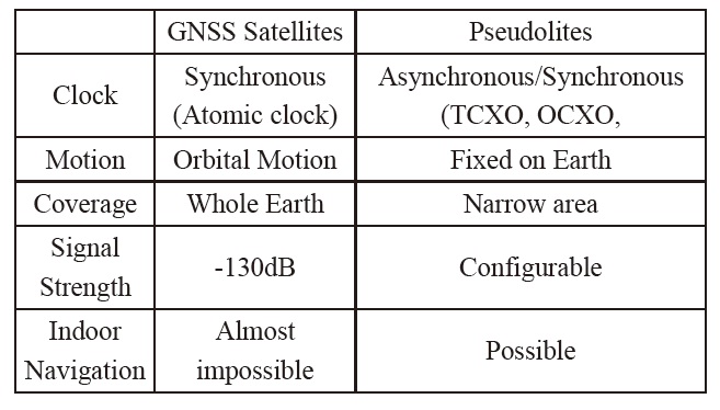
GNSS signals are too weak to be tracked indoors. Therefore, there have been several studies on the indoor positioning. Pseudolite-based navigation is one of the major approaches. Pseudolite is a signal transmitter that can be configured to emit GNSS-like signals for enhancing GNSS by providing increased accuracy, integrity, and availability [1]. Furthermore, an independent navigation system can be constructed using proper pseudolite constellations. Table 1 shows the differences between GNSS satellites and pseudolites.

Before using pseudolite signals for navigation, each position of the phase centers of the pseudolite antennas must be calibrated precisely. The calibration error will give biased positions in pseudolite-based navigation.

There have been several studies on the calibration method of pseudolite antenna position. Pseudolite-transceiverbased self-calibration methods using range rates [2] or distances [3] gave precise calibration results. However, these methods could not be applied to calibrate positions of normal transmitter-type pseudolites. For the calibration of pseudolite transmitters, there is a method based on an Inverted-GPS positioning algorithm, which uses carrier phase measurements collected at several known positions [4].

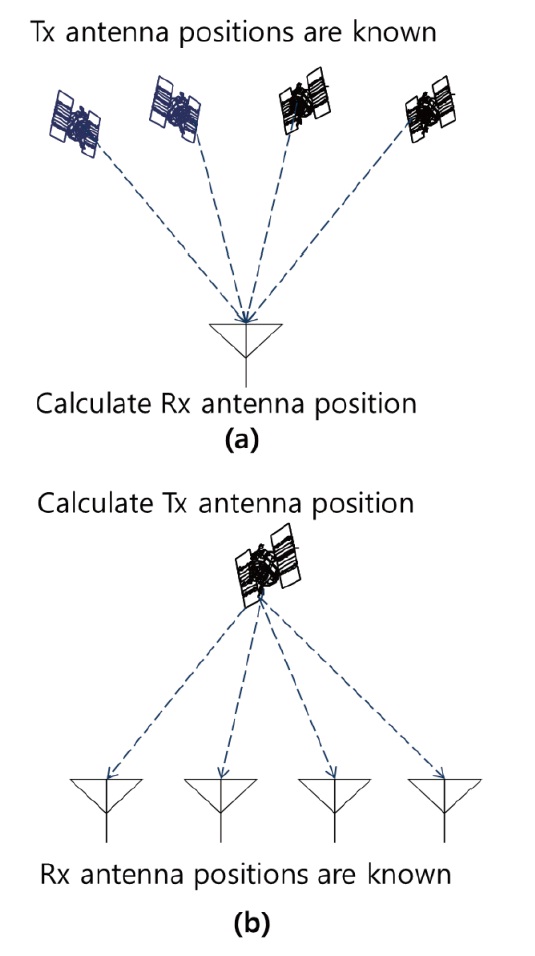
The conventional GPS algorithm calculates unknown RX antenna positions based on the measurements obtained from GPS signals transmitted from TX antennas whose positions

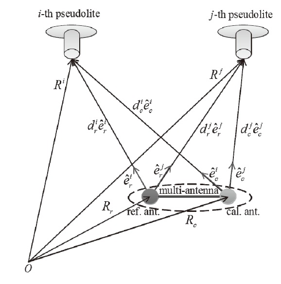
are known. On the other hand, the Inverted-GPS Positioning algorithm calculates unknown TX antenna positions based on the measurements obtained by RX antennas whose positions are known. Fig. 1 illustrates the conventional GPS method and the Inverted-GPS method.

Like GPS satellites, pseudolites provide both pseudorange and carrier phase measurements. A precise calibration of pseudolite position is possible using the Inverted-GPS Positioning algorithm with carrier phase measurements. To perform calibration, we have to collect carrier phase measurements fi rst. However, carrier phase measurement collection is a very diffi cult process due to cycle slips. Furthermore, there are other diffi culties such as the installation of calibration points and the placement of the antenna in exact positions to collect measurements.

Kee resolved the cycle ambiguity of carrier phase measurements by a simple method using a short baseline condition [4]. By using this condition, the ambiguity could be fi xed easily near a reference antenna. After that, the antenna is moved to a calibration point to collect carrier phase measurements. Th e short baseline condition made the ambiguity resolution very easy.

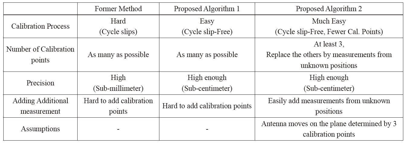
However, this method cannot be used if any cycle slips or loss of locks occur. In fact, this is a critical problem in real situations. To fix this problem, a new multi-antenna-based calibration method of pseudolite position is proposed in this paper. Moreover, an enhanced calibration method which uses measurements collected at unknown positions is proposed. By using these methods, more effi cient and easier calibration of pseudolite position is possible.

By double-diff erencing the carrier phase measurement s model equation, every pseudolite-related or receiver-related delay error is canceled out as in the following equation:

φ : carrier phase measurement

d : geometrical distance

N : integer cycle ambiguity

λ : wave length of carrier

ε_φ : noise of carrier phase measurement

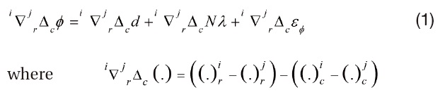
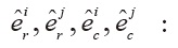
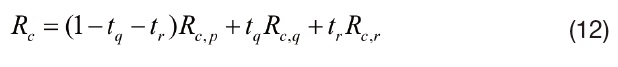
Double-differenced carrier phase (DDCP) measurement is composed of a geometrical distance term, a cycle ambiguity term, and a noise term as in equation (1). The superscripts i and j represent the i ? th and j ? th pseudolites, and the subscripts r and c represent the reference and calibration antennas. The geometrical relationship of the pseudolites and antennas is given in Fig. 2.

O : the origin of the coordinate system

Rⁱ, R^j : position vector of i ? th or j ? th pseudolite

R_r : position vector of reference antenna in multi-antenna

R_c : position vector of calibration antenna in multiantenna

unit Line-Of-Sight (LOS) vectors from reference or calibration antenna to i ? th or j ? th pseudolite

The multi-antenna is composed of a reference antenna and plural calibration antennas. The positions of each antenna segment are fixed relative to each other.

Dividing both sides of equation (1) by the wavelength of the carrier, we can rewrite the DDCP measurement equation as:

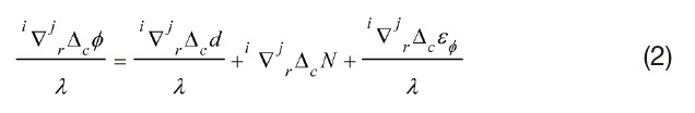
By rounding off both sides of equation (2), we can calculate the cycle ambiguity term very easily as:

but only if the following condition is satisfied:

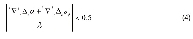
We assume a multi-antenna whose calibration antennas are placed within half a wavelength of carrier from the reference antenna. With this short baseline, the condition (4) generally holds with prevalent pseudolite geometry. Consequently, the ambiguity elimination can be done easily by the short baseline condition anytime and anywhere. This means the ambiguity value can be eliminated from the carrier phase measurement at each epoch by equation (3). Through this epoch-by-epoch ambiguity elimination, the change of ambiguity value between epochs due to cycle slips or losses of lock does not matter anymore.

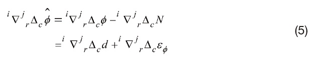
Now we can define the DDCP measurement whose cycle ambiguities are eliminated as follows:

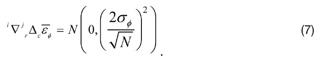
To improve the accuracy of pseudolite position calibration, we can average the ambiguity-eliminated DDCP measurements for N epochs as:

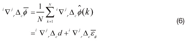
By averaging, the distribution of measurement noise becomes:

σ_φ denotes the standard deviation of carrier phase measurements. Equation (6) can be rewritten using position vectors and unit LOS vectors defined in Fig. 2 .

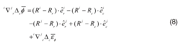
Now we can construct a navigation equation from equation (8) as equation (9).

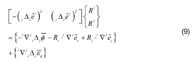
Considering l calibration points, m pseudolites, and n antennas in the multi-antenna, navigation equations can be formed in the same way. The following equation (10) shows the combined matrix equation.

The state vector x is composed of position vectors of pseudolite antennas. H_cal is the matrix composed of unit LOS vectors which are unknowns at the initial state. The Z_cal vector includes measurements and unit LOS vectors. v_cal is a measurement noise vector. The dimensions of each matrix and vector are shown in equation (11).

At first, we assume the initial pseudolite positions roughly to calculate the initial LOS vectors. Since the operating range is narrow, the initial guess of pseudolite antenna position is important. In this paper, we assumed that we can choose the initial guess of pseudolite antenna position within 1 meter from the true position using a tape measure.

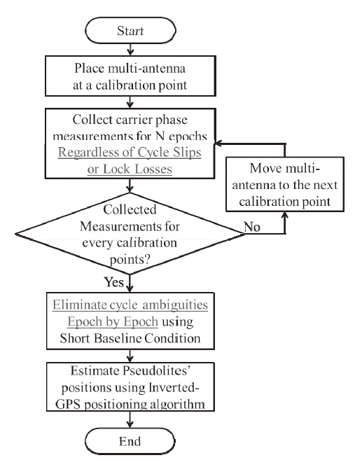
Then, the state vector can be estimated by iterative least square solutions. The overall calibration process is illustrated in Fig. 3.

Although the calibration process of pseudolite position becomes easier using algorithm 1, installing accurate calibration points and placing the multi-antenna at the exact calibration point are still difficult processes. Algorithm 2 is an enhanced method to reduce the number of calibration points needed for the calibration.

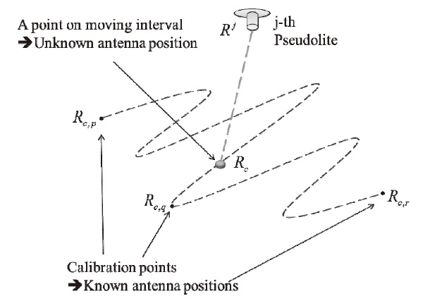
For algorithm 1, we utilized carrier phase measurements only collected at calibration points. However, for algorithm 2, we use the measurements collected while moving the multiantenna from one calibration point to another (at unknown antenna positions). As a result, it is possible to replace some measurements collected at calibration points by measurements collected while moving the multi-antenna.

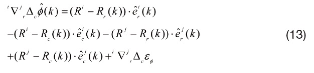
Generally, only measurements collected at known positions can be used to calibrate pseudolite position. To utilize measurements from unknown positions, a simple assumption should be applied. The antenna moves on the plane determined by three calibration points whose positions are known precisely. This assumption is true in many cases in which the operating area has flat floor. Fig. 4 illustrates this situation.

Let the position vector of the point on a moving interval be R_c, and the three calibration point position vectors be R_{c, p}, R_c,q and R_c,r. Then R_c can be expressed using R_{c, p}, R_c,q and R_c,

_r as in the following equation:

for some t_q and t_r. By substituting equation (12) into the DDCP measurement equation (8), a navigation equation can be obtained. The dummy variables t_q and t_r become additional state variables and can be estimated simultaneously with pseudolite positions. By the use of this method, the number of calibration points can be reduced down to three, which is the minimum number that can determine a plane.

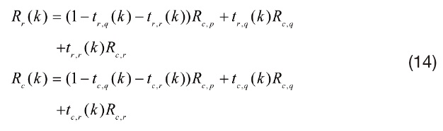
For algorithm 2, two kinds of carrier phase measurements are used to calibrate pseudolite position. One is measurements collected at calibration points, and the other is measurements collected at moving intervals with unknown positions. The former is processed in the same way as in algorithm 1 to build the navigation equation (10). For the latter, the elimination of ambiguity can be done in the same way. However, the building process of the navigation equation is different.

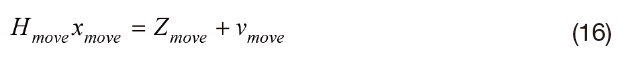
Firstly, we assume the number of epochs at unknown positions is K. Then the ambiguity-eliminated carrier phase measurement equation at the k ? th epoch is expressed as :

where 1 ≤ k ≤ K.

Assuming the reference antenna and calibration antenna move on the plane determined by three calibration points R_{c, p}, R_{c, q} and R_{c, r}, the reference antenna position at the k ? th epoch R_r(k)and the calibration antenna position R_c(k) can be expressed as :

t_{r, q}(k), t_{r, r}(k), t_{c, q}(k)and t_{c, r}(k) are unknown dummy variables at the k ? th epoch. Substituting equation (14) into (13) and collecting unknowns into state variables, we obtain the navigation equation for the k ? th epoch as follows :

We have measurements collected for K epochs, from m pseudolites, and by n antennas in the multi-antenna. Thus we can construct K(m ? 1)(n ? 1) navigation equations in the same way. Now we can combine these equations into a simple state equation. The states are pseudolite position vectors and dummy variables.

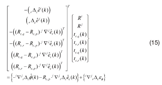
The state vector x_move is composed of position vectors of m pseudolite antennas and dummy values for each epoch. H_move is the matrix composed of unit LOS vectors which are unknowns at the initial state. The Z_move vector includes measurements and unit LOS vectors. v_move is a measurement noise vector. The dimensions of each matrix and vector are shown in equation (17).

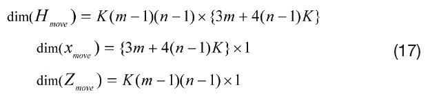
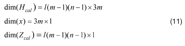
The navigation equations (10) and (16) can be combined as one matrix equation as follows :

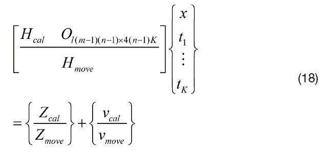
Equation (18) can be rewritten as equation (19) using matrices and vector symbols.

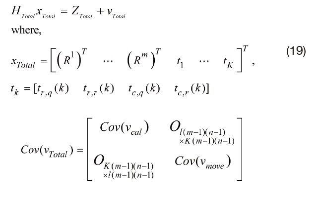
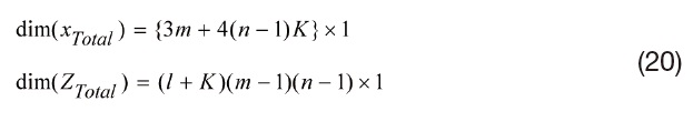
The dimensions of each matrix and vector are shown in equation (20).

Finally, the weighted least square solution is used to estimate the state vector

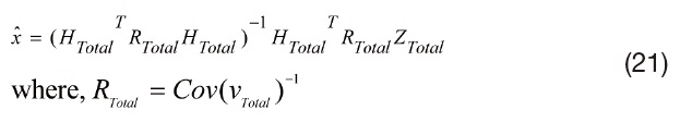
Using this result, we can build the H_Total matrix again, and then we can re-estimate the state vector

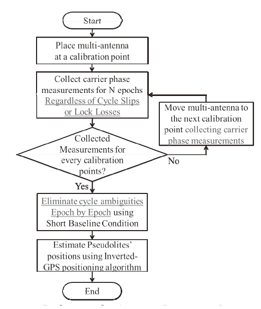
over and over again until the state vector converges. The overall calibration process is illustrated in Fig. 5.

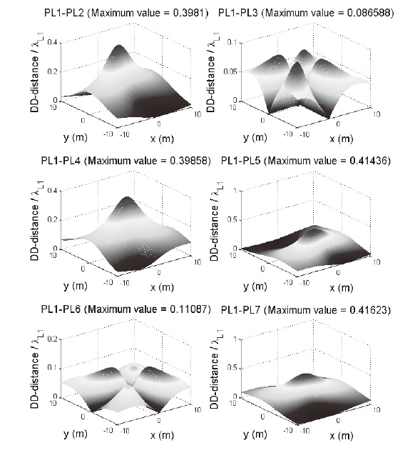
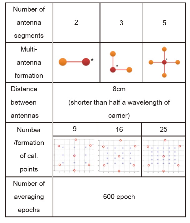
In algorithm 1, there is an assumption that the inequality (4) is always satisfied if the baseline is shorter than half a wavelength. A simulation is conducted to verify this assumption. Fig. 6 shows the pseudolite constellations.

The simulated values of

for every pseudolite

combination are given in Fig. 7. The reference pseudolite for double-difference is SV 1, which is placed at the center. At every simulated cell, the value was calculated to be smaller than 0.5. By this result, the ambiguity elimination can be successfully done using a short-baseline multi-antenna anytime and anywhere.

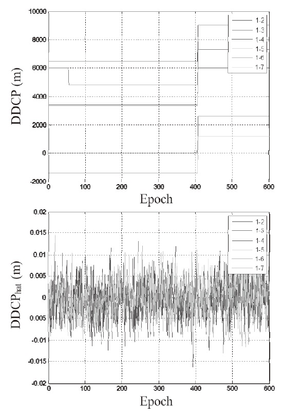
Now the ambiguity elimination algorithm is tested using simulated carrier phase measurements which include some cycle slips. The upper plot of Fig. 8 shows the doubledifferenced carrier phase measurements including cycle slips. The lower plot residual of double-differenced carrier phase measurements after applying the ambiguity elimination algorithm. There are no biases or discontinuities after ambiguity elimination, therefore we can use these measurements regardless of the integer cycle slips.

The calibration result is simulated in comparison with the previous method. Th e simulation environments are given in Table 2.

In the multi-antenna of Table 2, the antenna which is marked using asterisk is the reference antenna, and the other antennas are the calibration antennas. Calibration points are placed at equal intervals from about (-2.25, -1.5) to (2.25, 1.5) meters (roughly illustrated in Table 2).

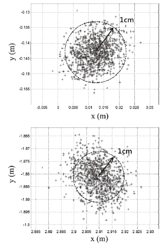
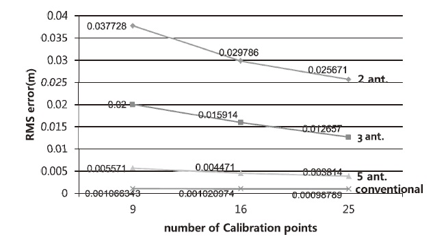
The pseudolite calibration is performed 1000 times for each pseudolite, and the RMS error is calculated. The centered pseudolite (SV 1) gave the smallest mean RMS error due to the geometry, and pseudolite placed at (3,-2) in Fig. 11 (SV 2) gave the biggest mean RMS error. Fig. 9 shows the best and worst results of the RMS errors. The upper figure is the result of SV1 and the lower one is that of SV2. 3 antennas and 9 calibration points are used. The blue points are the calculated pseudolite positions, and the red circles are the true pseudolite positions. The simulation result shows that the proposed algorithm works well and leaves small errors. The calibration error causes bias-type errors for users of pseudolite-based navigation. Th erefore, the calibration error must be suffi ciently small.

In the same way, every pseudolite position could be

calculated for 2/3/5 antennas and 9/16/25 calibration points. The averaged RMS errors are summarized as a graph in Fig.10.

The RMS error of the calibration of pseudolite position becomes smaller as the number of calibration points and antennas increases.

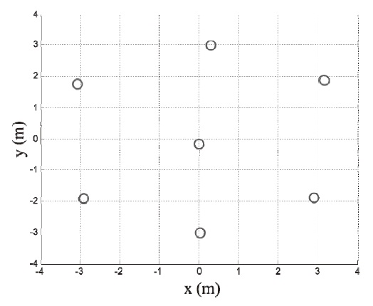
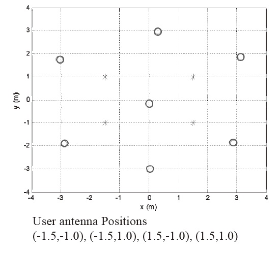
As shown in Fig. 10, the calibration result of the proposed method is slightly poorer than that of the conventional method. This seems to be due to the geometric weakness of the short baseline multi-antenna. However, what is important is not the accuracy of pseuodolite position, but the accuracy of positioning based onrated pseudolites. In this context, the position error is simulated when the pseudolite position has errors. User positions used in the simulation are given in Fig. 11. Asterisks represent user antenna positions, and circles represent pseudolite positions.

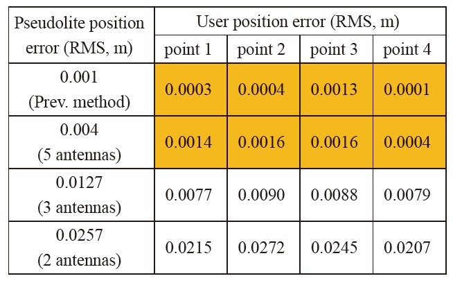
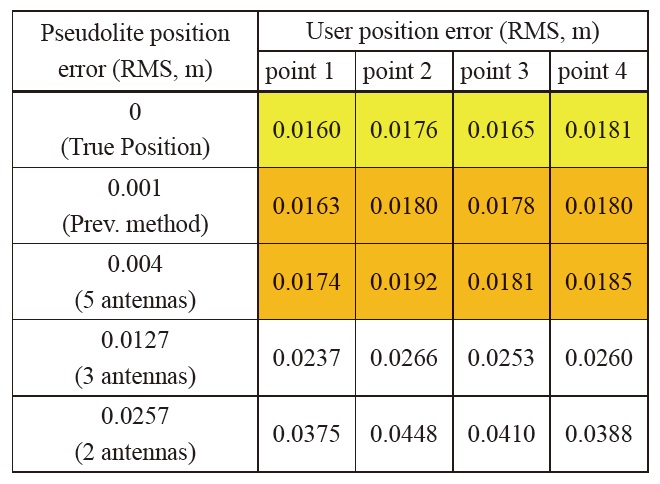
The user receiver calculates its position using a carrierphase- based GPS algorithm. The only error source included in the carrier phase measurements is thermal noise (2mm standard deviation). Therefore, we can see the effect of only the calibration error on the user position. The simulation is performed for various pseudolite position errors. The results are summarized in Table 3. Each value in Table 3 represents the mean RMS error value of 1000 simulation results.

The user navigation errors of the previous method and the proposed method (5 antennas) are calculated as similar values. From the ？ruePosition case, we can see that even when there is no calibration error, the navigation user has few centimeters of position error. This is due to the measurement noise. So the user position error due to the calibration error can be calculated by subtracting the error of the ？rue Position case from the other results in Table 3 as in Table 4.

We can see that there remains a negligible amount of errors. In most applications, these amounts of error do not matter at all. One of the strictest applications is indoor robot control. It requires centimeter-level accuracy. Therefore, the positioning error due to the pseudolite calibration must be about a few millimeters or even smaller. If we use the proposed algorithm with 5 antennas, this is satisfied. Consequently, the suggested calibration method causes no problems with respect to precision.

A simulation to show the feasibility of algorithm 2 is

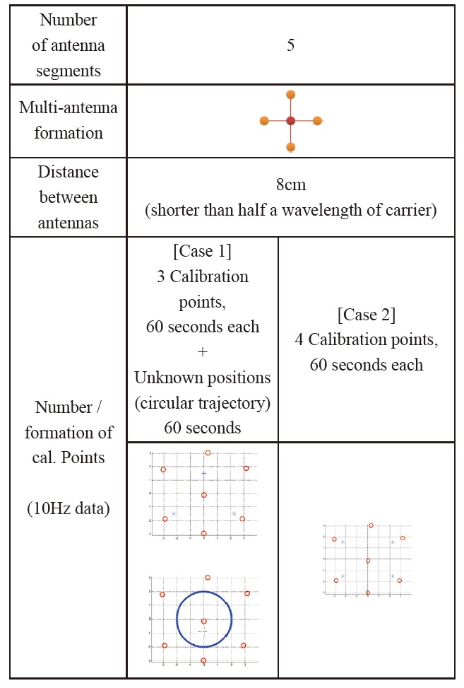
performed. Algorithm 2 utilizes measurements from unknown positions to replace calibration points. The simulation environments are given in Table 5.

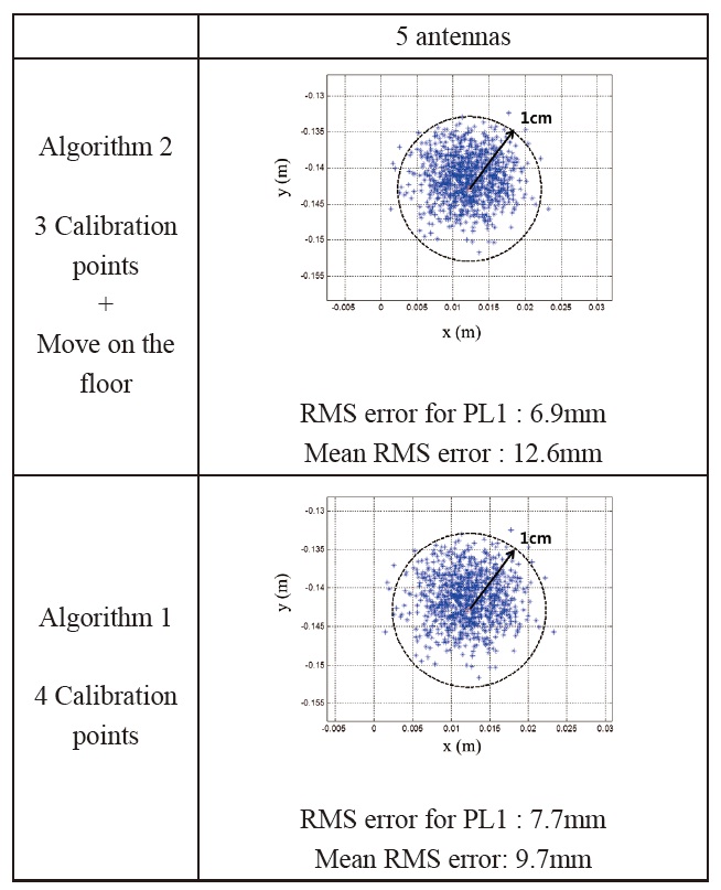
For case 1, the number of calibration points is the minimum, three. The measurements collected at unknown positions (circular move) are used together. Calibration points are placed at (0, 1.5), (-2.25, -1.5), and (2.25, -1.5). The radius of circular trajectory is 2 meters (roughly illustrated in Table 5).

For the comparison, a simulation for algorithm 1 is performed as well. Calibration points are placed at (2.25, 1.5), (2.25, -1.5), (-2.25, 1.5), and (-2.25, -1.5) meters (roughly illustrated in Table 5). The total number of measurements used in the calibration is set equal for both cases.

The simulation result shows that a calibration point could be replaced successfully by measurements collected from unknown positions and that algorithm 2 works. The precision of calibration is similar to that of algorithm 1. Strictly, the mean RMS error of algorithm 2 is slightly larger than that of algorithm 1. However, this small difference does not result in signifi cant error for the user, and it can be said that the precision of algorithm 2 is enough for most applications.

In actual calibration, the use of additional measurements is very easy for algorithm 2. It is not easy for algorithm 1, and very hard for the conventional method. Using more measurements, the calibration using algorithm 2 can easily achieve better precision than other methods.

Table 7 shows a summary of the simulation results. By using the proposed algorithm 1, the calibration process becomes easy due to the use of the multi-antenna, and the calibration result is suffi ciently precise.

In the case of algorithm 2, the calibration process becomes much easier, replacing the calibration points by measurements collected at unknown positions. The enhancement of precision by adding additional measurements is easy for algorithm 2. The assumption that the antenna moves on the plane determined by 3 calibration points should be satisfied.

Thus, if the floor of the navigation area is flat, we can use algorithm 2 and conduct the calibration very easily. If the floor is not fl at, algorithm 1 can be used.

To use pseudolite systems, the pseudolites own positions must be calibrated in advance. One previous study that used

a carrier-phase-based Inverted-GPS positioning algorithm, could not be applied to measurements including any cycle slips or losses of lock. For this reason, the previous method was considered to be inefficient, time-consuming, and inapplicable to ill-conditioned or wide areas.

In this context, this paper proposed a multi-antennabased pseudolite calibration algorithm. By using this method, the ambiguity can be eliminated, epoch-by-epoch easily. Hence, cycle slip-free carrier phase collection is possible. Moreover, an enhanced calibration algorithm is also proposed. This algorithm utilizes measurements collected at unknown positions to replace calibration points and minimize the number of calibration points down to three. The measurement can be collected easily assuming planar positioning of the calibration points.

Simulation results were given to show the feasibility of the proposed algorithm. According to the simulation result for algorithm 1, the calibration accuracy of the proposed method was calculated as for the case of 5 antennas. However the actual navigation user error was almost the same as that of the previous method. The calibration process becomes remarkably easy and convenient using algorithm 1. The simulation results for algorithm 2 show that it is possible to replace the calibration points by use of measurements from unknown positions. The precision of algorithm 2 is similar to that of algorithm 1. Using algorithm 2, the calibration process becomes even easier than algorithm 1.

In the case of actual calibration, algorithm 2 can easily be used if the navigation area has a flat floor. In the other general cases, algorithm 1 can be used to make the calibration process easy and convenient.