The influence of automation on the operation and the design of technical processes have increased progressively. Therefore, process and its control become autonomous units. Fly-by-wire aircraft and vehicles are the representative system. Here, not only the control tasks itself but also the reliability and safety depend on the correct functioning of all process parts, actuators, sensors and control computers. Faults in the system must then immediately be displayed to the operator and redundant or reconfigurable components must be activated by a fault management system for critical processes. The autonomous fault detection algorithm in the past was mostly realized by limit checking of some important process variables. This is in many cases sufficient to prevent larger failures or damages. However, faults are detected rather lately and a detailed fault diagnosis is usually impossible with this simple method. Thus, numerical techniques based on a system model and artificial intelligent methods are well established and have been written, such as Chen and Patton (1999), Isermann(2006). This paper is focused on the signal based fault detection process by PCA (Principal Component Analysis).
PCA has been applied successfully in the monitoring of complex systems (Pessel 2007, Ma 2009, Tharrault 2008, Chiang and Colegrove 2007, Kano and Nakagawa, 2008). It is attractive that the available process measurements are highly correlated but only a small number of events produce unusual patterns. Indeed, PCA transforms the data to a smaller set of variables which are linear combinations of the original variables while retaining as much information as possible. The largest principal component analysis corresponds to the direction in which the projected observations have the largest variation. The second largest principal component is then orthogonal to the largest one and again maximizes the variance of the data points projected on it. From a regression point of view, PCA also constructs the optimal orthogonal linear projections from the eigenvectors of the data covariance matrix.
In practice, conventional PCA methods are widely researched to detect the fault of the mechanical system (Chen 1999, Pessel 2007, Tharrault 2008). However, conventional PCA methods do not consider the fault detection of the dynamic system like the vehicle sensor unit. The fault detection performance of a sensor unit is decreased by the effect of system movement. To avoid this effect, the modified PCA method is proposed in order to obtain the processed result that is not influenced in the dynamic environment.
When the fault occurs in the dynamic environment, it is impossible for conventional PCA to classify the fault pattern in the sensor data because motion of the vehicle also makes the similar pattern(Ed. note: This is confusing. Please clarify). Consequently, we cannot decide which pattern is made by a fault or which one is the result of sensor motion. This means that PCA methods are not available when the sensor module is moving. In this paper, for that reason, parity space analysis is additionally used with the PCA method. As parity space approach is one of the generally used fault detection algorithms it is reported by Potter (1977), Zhang (1999), Ragot (1991) and Ray (1991). They have introduced a null space matrix to compute the parity vector. Using the matrix, it is possible to cancel the motion effect on the input of PCA methods by simple algebraic calculation. Thus, the parity space approach combined with PCA, known as modified PCA, is independent of sensor module movement and it also provides fault detection without heavy computation power. The main step of this algorithm is divided into two stages. One is to compute the parity vector in which the sensor data does not include movement of the system. And the second step is to generate a fault pattern that can be separated from the normal sensor pattern. In the simulation, redundant IMU, which has 6 sensors (Seong Yun Cho 2004, 2005), is used and fault pattern recognition are achieved by EM which is a popular numerical method for location modes of likelihood functions as shown by Bishop (2006) and Han (2009)
Therefore, this paper aims to develop a modified PCA method that combines the advantages of PCA with the parity space approach to improve its performance. PCA is mainly used to detect the fault and the modified PCA relies on applying the parity space approach to remove the sensor movement.
The outline of the paper is as follows: In section 2, a brief description of the PCA is presented using vector signal input. Furthermore, section 3 discusses a derivation of modified PCA equations and a specification about the fault detection scheme using modified PCA. In section 4 the simulation for redundant IMU is introduced and we show that modified PCA is demonstrated through an example. Lastly, section 5 discusses the concluding remarks.
2. Principal Component Analysis
PCA is a way of identifying patterns in data, and expressing the data in such a way as to highlight their similarities and differences since patterns in data can be difficult to find in data of high dimension, i.e. by reducing the number of dimensions, without much loss of information. This technique generally is used in image compression.
First of all, each of the data has to subtract the mean value. The mean subtracted is the average across each dimension. So, all the values have the mean of all the data points subtracted, and all the values are subtracted from them. This produces a data set whose mean is zero.
where
And the eigenvalues and eigenvectors of the covariance matrix can be computed as follows,

where

where
In this paper, the 2 dimensional feature vector of the sensor data covariance matrix is used. This means some information is missed. The final data set will have fewer dimensions than the original. A feature vector is constructed by taking the two biggest eigenvectors, and forming a matrix with these eigenvectors in the columns,

where,
3. Proposed Fault Detection Algorithm
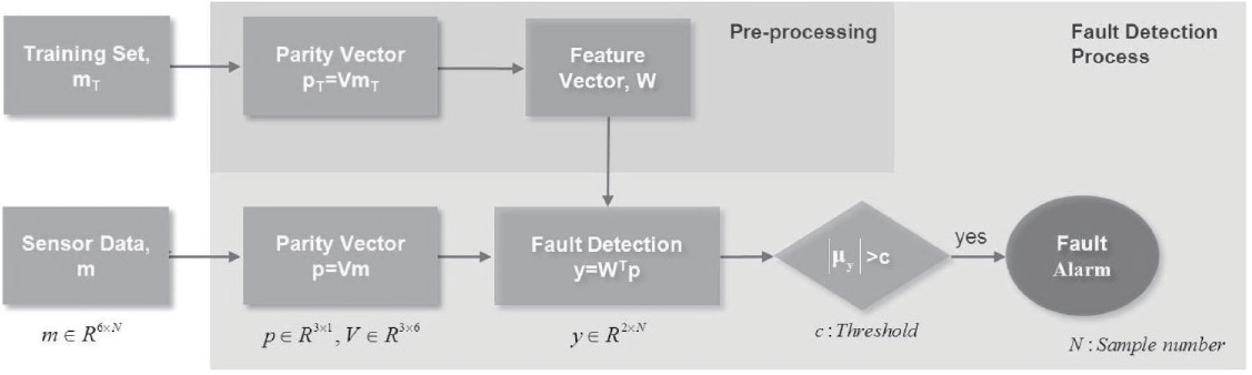
As we mentioned above, PCA is an attractive technique to detect the fault of the satellite attitude control system. The satellite has redundant inertial sensors and these are a hotstandby type hardware redundancy. Therefore, all sensor data can be can acquired during each step and all of them are used to calculate a principal component and a feature vector. The calculated feature vector is used to make a pattern through transposing the original data set to the feature plane. Then, the faulty sensor’s pattern will be separated with the normal sensor’s pattern. The main process for the modified PCA is similar to conventional PCA. But modified PCA calculates the feature vector just one-time using a training set unlike conventional PCA. This feature vector represents only the normal sensor output. On the contrary, the fault mixed sensor data makes another processed result. It is the reason why the fault can be detected with normal sensor data. Thus, the effect of moving motion, which creates a different pattern, must be removed. The parity space concept helps to remove the negative effect from the movement. The fault detection process of modified PCA is shown in Fig 1. It is mainly divided by two steps, pre-processing and the online fault detection process.
3.1 Modified PCA using Parity Space Concept
The measurement of inertial sensor module with N sensors are defined as
Definition 1 The matrix


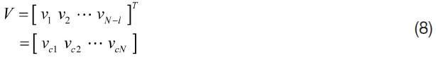
where
Definition 2 The column space of matrix
Definition 3 The parity vector is defined by
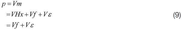

where
Definition 4 The columns of
The feature vector, which is not influenced by sensor movement, is generated using parity vector
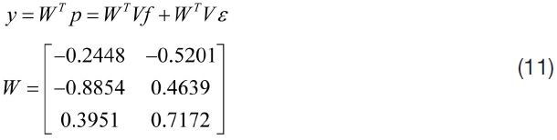
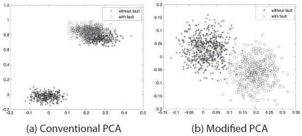
Fig. 2 presents the difference of the generated pattern between the modified PCA and conventional PCA when redundant IMU is moving. Due to the dynamic motion of the sensor, the conventional PCA generates a pattern similar to the sensor fault situation. (Please clarify). Therefore, the moving motion of redundant IMU affects the position of patterns as shown in Fig. 2(a). It makes it difficult to classify the fault pattern from the output of the moving sensor module. On the other hand, the modified PCA is not affected by the moving motion redundant IMU like Fig. 2(b). With this, the modified PCA is more adequate for fault detection compared to conventional PCA.
3.2 Fault Detection Scheme Using Modified PCA
Sensor fault detection is based on a similarity test between the fault free pre-processed and real time generated pattern with the modified PCA. The feature vector would be calculated ahead of the fault detection process. And the real time pattern generation step occurs next. The judgement of fault occurrence is the third step. Thus, to detect the fault, first the sensor data which does not have fault, which we call the training set, is obtained from the sensor module. This process must be guaranteed fault free sensor data because the fault mixed sensor data cannot represent the normal sensor pattern. The generated training set is used to shifting the measurement space to parity space. At this time, 6 dimensions of sensor data is reduced to 3 dimensions because of the inner product with matrix V and the sensor data. The feature vector can be computed using the training set data in parity space. Using the computed feature vector, the normal sensor pattern can be made easily. For convenience, the mean of this pattern translates to (0, 0) on the feature plane, which consists of coordinates with principal component vectors. This process is followed for fault detection and we call that the “pre-processing” process.
In the preparation step for fault detection, a feature vector,
4.1 Redundant IMU Data Generation
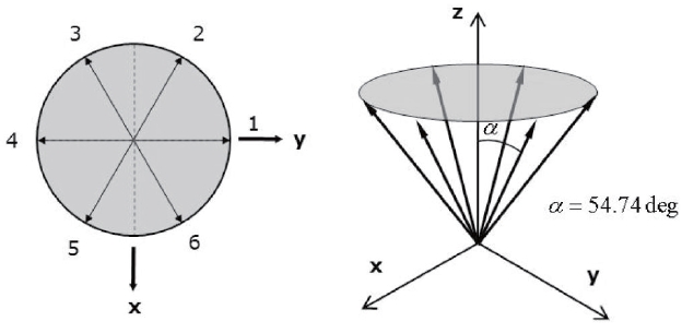
The redundant IMUs are discussed extensively by Seong Yun Cho (2004, 2005) and Sturza (1988). In redundant IMU, two orthogonal IMUs are implemented. Therefore, the redundant IMU has enough numbers of redundant components. It is possible to calculate and reconfigure the redundant IMU body coordinate output if half of the redundant IMU sensors are available. Each sensor is continuously operated. This means that the redundant IMU used in this paper has dynamic redundancy by using hat standby. The redundant IMU has its own configuration as shown in Fig. 3. It affects not only the relationship between each sensor coordinate and body axis but also the fault detection performance of the redundant IMU. Gyros and accelerometers used in the redundant IMU have a coneshape arrangement. Each sensor tilts 54.74 degrees against the z-axis and is configured as having an equal angle on the x-y plane. Generally, it is already known that the cone-shape
redundant IMU is the optimal configuration for FDI.
Redundant IMU used in this paper consists of low-grade MEMS inertial sensors. The Fault detection algorithm for this is almost the same, though they are not used in the real attitude control system in the satellite. The error model for the redundant IMU is designed by considering three error factors, misalignment error, bias, and scale factor as in (12). They are the representative error source of MEMS grade sensors. Misalignment error is a miss attached value of the sensor at the pre-defined coordinate. Bias and scale factor are the values which are calculated for each sensor. Equation (12) represents the redundant IMU signal model when two orthogonal IMUs were used.
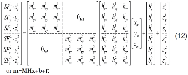
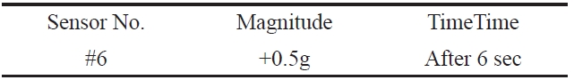
where m is a measurement of each gyro sensor and accelerometer, M means the misalignment correction matrix, H is the measurement matrix which is the geometry relationship between the sensor and the redundant IMU module, x represents redundant IMU output, b is bias, and ? is sensor noise. Here, M and b are calculated by calibration of the sensor module and H is defined mathematically. Using measurement equation (12), A redundant IMU sensor signal is generated. The sensor output is used the accelerometer measurement of the redundant IMU in the simulation. It makes 100 outputs every second. An additive fault is considered, which is similar to the bias component. Fault configuration is demonstrated in Table. 1. The dynamic situation of redundant IMU is configured. The size of dynamic motion is a relatively big component compared to fault size. This assumption is due to confirm the fact that the proposed fault detection method works well in the dynamic environment.
[Table 1.] Fault configuration

Fault configuration
[Table 2.] Movement of satellite
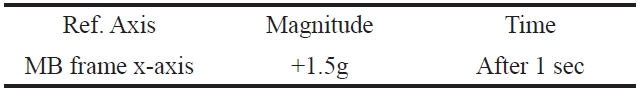
Movement of satellite
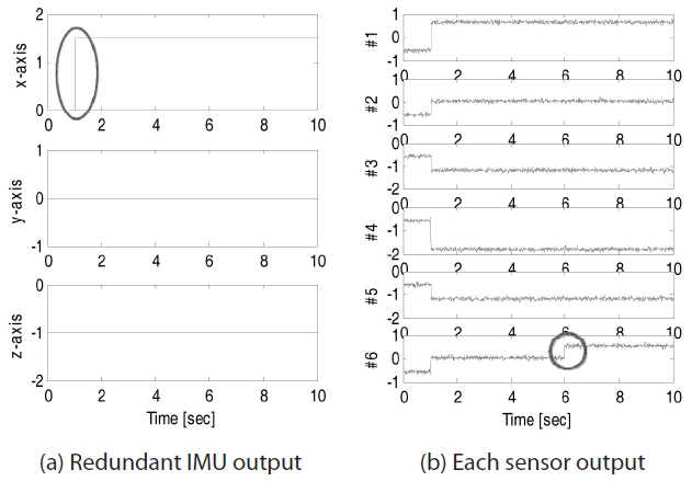
In this section, the performance of the proposed fault detection algorithm developed using the modified PCA and EM is illustrated. The data used in this simulation are generated as mentioned above. 1,000 signal samples of the redundant IMU are used as the deterministic input to the fault detection process. The measurement noise variances are used in the experiment result of real sensor outputs. Sensor data contains dynamic motion of the satellite at 1 sec as shown in Fig 4(a). Fig. 4(b) shows the 6-th sensor output mixed fault at 6 sec and dynamic motion is generated at 1 sec.
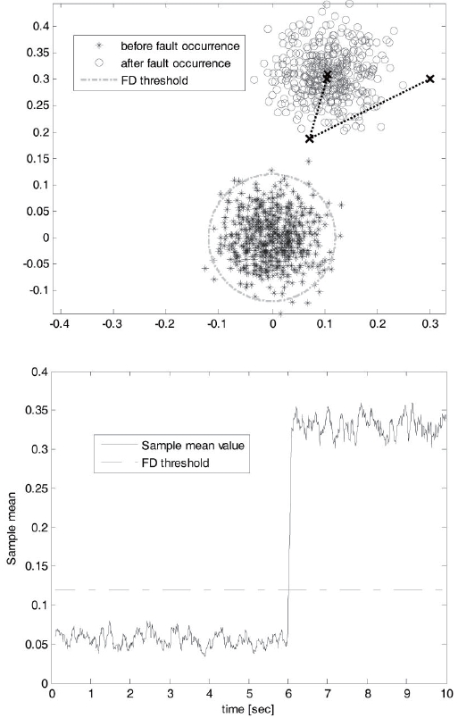
The fault classification result of the proposed fault detection algorithm is shown in Fig. 5. Each small circle signifies the result of the modified PCA at each time step. As previously mentioned in Fig. 2, it was impossible for conventional PCA to classify the moving motion and fault effect. Otherwise, the modified PCA can separate them because parity space removed the negative effect due to the dynamic motion. This characteristic helps us to concentrate only fault pattern detecting. The result of the modified PCA does not change enough to be considered as a fault pattern at 1 sec. At 6 sec, the pattern moved to another position on the feature plane. The calculated feature vector in the preprocessing step cannot represent fault of the sensor output. That is the reason why we emphasize the fault free training
set. As use warranted fault free sensor data, a feature vector just represents normal sensor data. Faulty sensor output has a principal component, which represents fault because fault is generally much larger than measurement noise. Therefore, the defined principal component of normal sensor data can no longer be the principal component. Therefore, the mean of generated pattern is moved to some position. (Ed. note: Please review and clarify). As a result it provides us with evidence to detect a fault.
The simulated result shows more specific evidence about the performance of the proposed modified PCA method. Until 6 sec, the pattern mean of sensor data is located around (0.0). It is always placed in the small variation boundary, threshold, from (0, 0). The position of normal sensor pattern mean is located on (0, 0). Consequently, we can regard the redundant IMU as normal. In opposition, the pattern mean moves around (0.1059, 0.3096) after 6 sec from operation. This value is big enough to consider that the fault occurred because it is bigger than the threshold. For that reason, we can only know that
The fault makes the difference for the pattern if the modified PCA is used for fault detection. And the EM algorithm is possible to classify the each pattern mean location. (Ed. note: This is confusing. Please clarify). The dotted line is the iteration process to compute the mean of the pattern. From using the modified PCA method, it is expected that the 6-th sensor has a fault and it is estimated immediately after the fault occurs.
PCA is a powerful fault detection method. However, the conventional PCA, which is based on the estimation of the sample mean and covariance matrix of the data, can cause considerable error in the inertial sensor fault detection because of system movement. Therefore, it is impossible to use the conventional PCA method for the satellite inertial sensor unit. As a sensor is moving, principal components of the sensor data covariance matrix would be changed. In addition, the PCA processed result of the training set also cannot represent the normal sensor because of the effect of movement. To remove this negative effect of sensor movement, this paper proposed the modified PCA. The modified PCA basically consists of the PCA and parity space approach. PCA provides a theoretical base to detect the sensor fault and the parity space approach is additionally used with PCA to improve the fault detection performance. The objective of the parity space approach is to generate the pattern which is not changed when the sensor moves. The effect of the sensor movement can be caused by matrix
The performance of the developed fault detection algorithm using the modified PCA is illustrated through a simulated example that shows its advantages. When the 6-th accelerometer of the redundant IMU has an additive fault of 0.5g, the modified PCA can detect the fault pattern although the sizes of sensor moving motion are bigger than the fault. The additive fault pattern was positioned around (0.1965, -0.0594) and it is the value over the threshold. From using the modified PCA method, it was possible to detect the fault of the moving redundant IMU.