The Sun presents variability in several timescales, ranging from days to several hundreds of years. The pe-riodic characteristic of solar activity has been studied in great detail (Chang 2007, 2008, 2009, 2011, Usoskin 2008). In particular, prediction of solar variation has become an extremely hot topic, in view of space weather fore-casting, encompassing a very wide variety of prediction methods and many different timescales (Petrovay 2010). The methods are mainly categorized into three groups: Precursor methods, Extrapolation methods, and Model-based methods.

It is evident that the sunspot cycle is rather irregular. The mean length of the most well-known cycle is ~11 years (a half of Hale's ~22 year periodicity), with a stan-dard deviation of ~1 year. The profile of sunspot cycles is asymmetrical, e.g., the rise is faster than the decay. That is, the solar activity maximum occurs 3 to 4 years after the minimum, while it takes another 7-8 years to reach the next minimum. It has been noticed that the length of the rise phase anticorrelates with the maximal value of solar activity. Historically, the relation was first formulated by Waldmeier (1935) as an inverse correlation between the rise time and the cycle amplitude. The observed anticor-relation between rise time and maximum cycle amplitude is approximately linear (Lantos 2000). A more significant anticorrelation between the cycle amplitude and the length of the 'previous' cycle was reported by Hathaway et al. (1994), who also showed a weaker anticorrelation between the decay time and the cycle amplitude. An an-ticorrelation between cycle length and amplitude can be understood as a characteristic of a class of stochastically forced nonlinear oscillators. Indeed, it can be reproduced by introducing a stochastic forcing in dynamo models (Charbonneau & Dikpati 2000).

In this paper, we investigate the sunspot area data spanning from solar cycles 1 to 23 by employing the Hil-bert transform technique. The Hilbert transform analysis is used to analyze variations of phase and amplitude of a local wave field (Komm et al. 2001). Instead of measuring time intervals and amplitudes of the solar activity within a predetermined duration, such as a length of ~11 years, we attempt to analyze sunspot area data as a deformed oscillator using the proposed method. This is possible in the sense that one of the most important advantages of using Hilbert transform is that one can study associations between the amplitude and the phase over various tim-escales. Once we demonstrate its availability in this pilot study, we will develop the method to extend to a predic-tion algorithm, and discuss it elsewhere.

This paper begins with descriptions of data and a pro-cedure by which sunspot area data is transformed in Sec-tion 2. We present and discuss results obtained with the Hilbert transform technique in Section 3. Finally, we dis-cuss and conclude in Section 4.

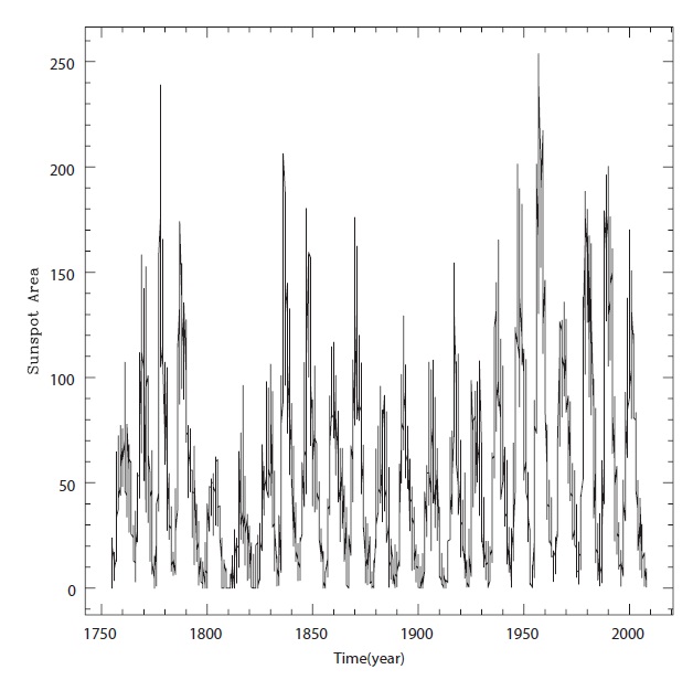
Despite its somewhat arbitrary construction, the time series of sunspot data is the longest homogeneous global indicator of solar activity. As shown in Fig. 1, for the pres-

ent analysis we have used the monthly sunspot area data from solar cycles 1 (March 1755) to 23 (December 2010), taken from the NASA website¹.

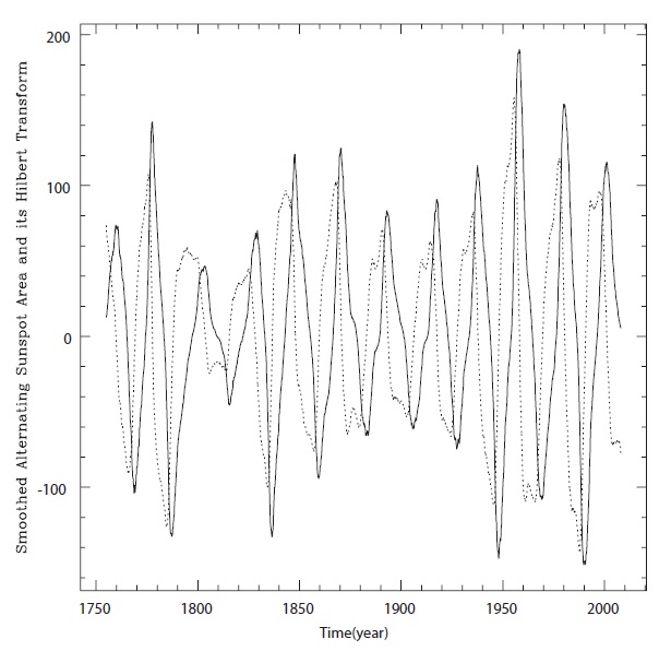
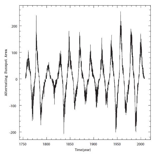
There is an alternative way of plotting the sunspot se-ries, in which alternating signs are given to successive ~11-year cycles (Bracewell 1953). In Fig. 2 we show the alternating sunspot area as a function of time, whose period is ~22 years rather than ~11 years. Instead of the 'raw' sunspot area series, many authors have found the alternating cycle convenient, but the idea has not yet been widely adopted. The basic idea for this alternation is based on Hale's well known polarity rule, implying that the period of the solar cycle is actually ~22 years rather than ~11 years. Alternating the 'raw' sunspot series is also well motivated from the physical point of view that attri-butes an alternating sign to even and odd Schwabe cycles (Bracewell 1953, 1986). Even though the time series of the sunspot area is a somewhat arbitrary construct, there may be an underlying physical quantity. The toroidal magnetic field strength B, or the magnetic energy, pro-portional to B², can be such a quantity, which is related to it in some nonlinear fashion (Passos & Lopes 2011). This representation is called the Bracewell transform, after Bracewell, who first suggested it (Bracewell 1953). Besides this physical reasoning, in this analysis this modification is a most helpful adaptation to the method of the pro-posed analysis.

1http://solarscience.msfc.nasa.gov/greenwch.shtml

There is a well-known mathematical technique for ex-tracting the instantaneous amplitude and instantaneous phase from oscillating data, which is well-defined and widely used in practice. This is the Hilbert transform. The underlying idea for this method is to represent a real os-cillating quantity by a complex function whose real part varies with time.

For a function x(t), its Hilbert transform

is de-fined by

where P is the Cauchy principal value of the singular inte-gral. With the Hilbert transform

of the function x(t), we obtain the analytic complex function, z(t), as

where

Thus, the instantaneous amplitude a(t) and the instantaneous phase

are given by-

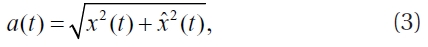
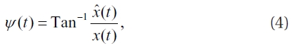
respectively. Subsequently, the instantaneous frequen-cy ω(t) and the instantaneous period T(t) are simply

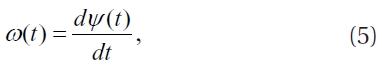
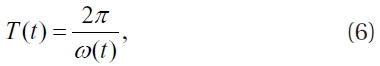
respectively.

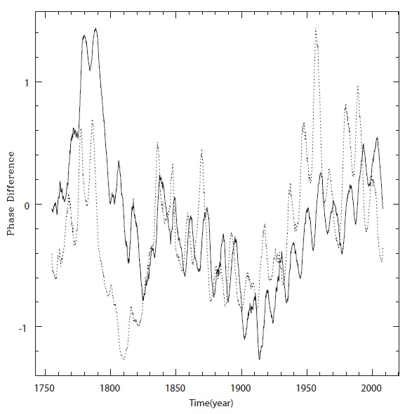
In Fig. 3, we show the smoothed alternating sunspot area in a solid curve and its Hilbert transform in a dot-ted curve. To get eliminate the arbitrariness of calendar years, we follow a standard practice, which is to adopt a moving-average using 11-year boxcar averages of the monthly averaged sunspot areas. Using Hilbert trans-form, one may immediately obtain the instantaneous amplitude a(t) and the instantaneous phase ψ(t) with the equations given above. In Fig. 4 we show the instanta-neous amplitude as defined by Eq. (3). The envelope of a sinusoidal function of ~22 year periodicity can be clearly seen. Other previously reported longer periodicities, such as, Gleissberg period (~70-100 years), can also be found, though it is not as straightforward as the obvious ~22-year periodic behavior. What is shown with the solid curve in Fig. 5 is the difference between ψ(t) defined by Eq. (4) and the straight line representing a linear phase of 22-year pe-riodicity over the observing duration. That is, the phase difference is given by ψ(t) - ω₀t, where ω₀ is a reference frequency that would be chosen as the angular frequency corresponding to the period of ~22 years. For compari-son, we also show the instantaneous amplitude function in the dotted curve after scaling with an arbitrary fac-tor. The phase difference appears to correlate with the

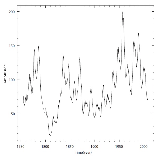
instantaneous amplitude. The correlation is not perfect, but general trends seem noticeable. That is, when a par-ticular solar cycle is strong, the value of the phase differ-ence becomes large, and vice versa. What this means is that in the strong cycle the phase advances ahead, and vice versa, as if the solar cycle remembers a 'correct' phase (Udny Yule 1927, Dicke 1978). This finding also supports the previously claimed anticorrelation between

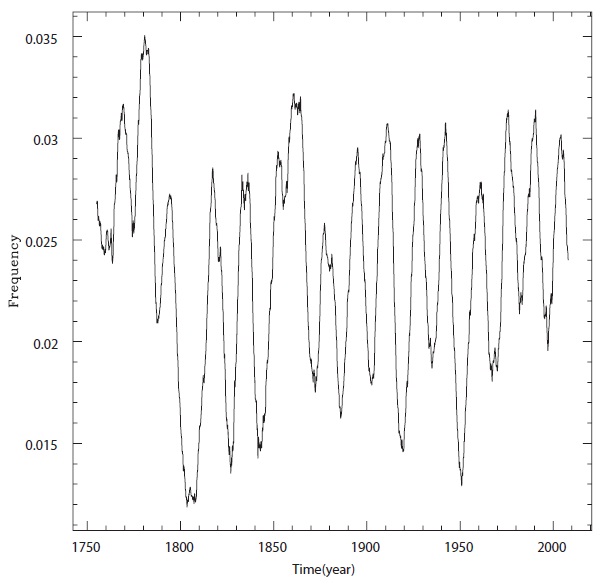
the cycle length and the maximum value of the solar cycle (Waldmeier 1935). In Fig. 6, we show the derivative of the instantaneous phase, which is the reciprocal of the peri-od. As seen in Fig. 6, on the other hand, the association of the instantaneous frequency given by Eq. (5) with the in-stantaneous amplitude is far less obvious. In the first half of the total duration (1750-~1870) it apparently behaves similarly to the instantaneous amplitude function. But in the second half (~1870-2010) no resemblance can be found. This is somewhat unexpected, since, according to the Waldmeier effect, one may expect some kinds of cor-related behavior between the instantaneous frequency and the instantaneous amplitude, at least in a timescale of ~11 years. We are currently investigating our find-ings and previous claims. This unexpected discrepancy should be explained in a further analysis of the currently proposed method.

We have attempted to analyze the observed sunspot data spanning from solar cycles 1 (March 1755) to 23 (De-cember 2010) by employing the Hilbert transform analy-sis method, which of the three main categories of predic-tion methods is considered an extrapolation method. One of the most important advantages in doing so is that the study of associations between the amplitude and the phase in various timescales is possible. In this pilot study, we adopt the alternating sunspot area as a function of time, as introduced by Bracewell (1953). This representa-tion has an advantage in the sense that it is physically mo-tivated and is suitable to the Hilbert transform analysis method suggested in this paper.

We have demonstrated that the instantaneous ampli-tude function clearly has a ~22-year periodicity (Hale's periodicity). Other longer periodicities, such as the Glei-ssberg period (~70-100 years), can also be seen. However, a shorter periodicity cannot be seen unless one utilizes another step for further Investigations. We also show that the phase difference apparently correlates with the in-stantaneous amplitude. On the other hand, however, we cannot find any obvious association of the instantaneous frequency and the instantaneous amplitude.

For forecasting space weather and understanding the solar magnetic field, studying solar activity is of great importance. Our ultimate goal in this study is to develop an algorithm that can be used to predict the solar activ-ity in various timescales at the same time. Rather than examining possible associations of the amplitude with other properties of solar activity over different timescales separately, as is commonly done, we are utilizing the Hilbert transform method as a consistent tool that can be adjusted in the timescale of interest. We are going to use phase information to estimate the amplitude of so-lar activity over various timescales. We have succeeded in simultaneously extracting the instantaneous amplitude and instantaneous phase information from the solar ac-tivity data. We are currently carrying out further analyses of the method to thoroughly understand it; for example, to determine why the unexpected discrepancy we dis-cussed above occurred. Having sufficiently understood the method, we may further refine the suggested method in developing an algorithm for solar activity prediction.