Optical interferometry has benefitted significantly from increased sensitivity, spatial resolution, and spectral resolution. Similarly, the capabilities of optical polarime-ters have also improved greatly in terms of sensitivity and spectral resolution. The next logical step is to combine long-baseline optical interferometry with polarimetry, which is called full-Stokes optical interferometric polar-imetry (OIP; Elias et al. 2008).
Full-Stokes OIP beam combiners can be added to ex-isting optical interferometers to obtain simple yet signifi-cant results (Elias 2004b). CHARA has an OIP beam com-biner that is undergoing testing (Mourard et al. 2008), but it is not a full-Stokes instrument. Design and operational experience with a simple full-Stokes OIP instrument will benefit the next generation of interferometers for OIP as well as scalar (~Stokes I) observations with improved cali-bration.
In this paper, we present scientific projects to demon-strate the benefits of OIP. They represent a small subset of many others. We present updated requirements and a preliminary full-Stokes beam combiner designs. One em-ploys simple optics and a sequential polarimeter, while the other is a bit more complicated and includes a simultaneous polarization capability. We also discuss a prelimi-nary end-to-end design for data reduction, including co-herent averaging, calibration, and imaging. In addition, we present a reimaged Be star model, employing a realis-tic number of telescopes and noise, based on part of the data-reduction design.
There are a number of possible OIP scientific projects (Elias et al. 2008) that involve scattering and/or magnetic interactions. In this paper, we highlight four of them.
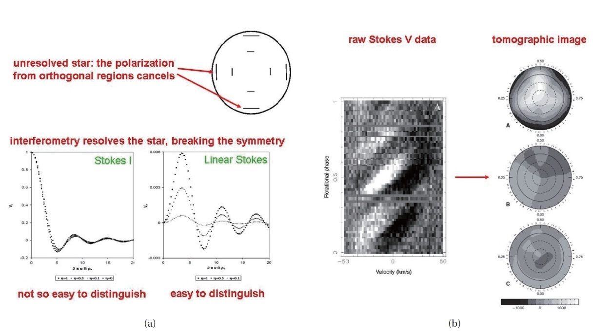
Consider an early-type star with a spherically sym-metric Thomson scattering atmosphere (Chandrasekhar 1950). Such stars are intrinsically unpolarized when ob-served with classical polarimeters because of azimuthal symmetry, and the magnitude of the polarization in-creases toward the limb (Fig. 1a). OIP breaks the symme-try (Elias 2004b), thus making even previously uninterest-ing calibrator stars interesting. The polarized visibilities provide better information on the stellar structure than Stokes I visibilities. There is very little difference between the three models for Stokes I visibilities (hard to mea-sure), even for large spatial frequencies, but for linear Stokes visibilities the differences are quite clear (Fig. 1a).
Late-type stars exhibit magnetically induced polariza-tion from Zeeman splitting. Such observations indicate how these objects produce magnetic fields in their inte-riors. Fully convective stars can create large-scale fields without differential rotation, which is inconsistent with existing models. Donati et al. (2006) mapped the magnet-ic fields of these stars with imaging tomography from po-larization time series (Fig. 1b). The rotational phase ver-sus velocity diagram in the Stokes V parameter show the positive and negative Zeeman components, which can
be converted to tomographic model images of magnetic fields. OIP observations of the stellar surfaces will directly confirm Zeeman splitting measurements.
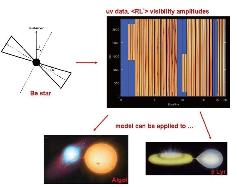
Just as with OB stars, the polarization of Be stars is also produced by Thomson scattering, but it comes from an axisymmetric disk orbiting the star. Classical polarim-eters detect polarization from these objects at the ~1% level due to the flattened disk geometry (as long as it is not viewed face on). Hα emission, acting as a tracer of the disk shape and angular size, has been observed with clas-sical optical interferometers (Quirrenbach et al. 1997). OIP measurements, however, will provide even more in-formation because continuum radiation dominates the disk environment compared to line emission.
Mackay et al. (2009) has shown how synthesized vis-ibilities of Be stars depend on parameters from a simple geometric model and a more detailed radiative transfer model. At 2.2 ㎛, the polarized Stokes visibilities (nor-malized) range from 10-2-10-3 for short baselines and 10-3-10-4 for long ones. In Fig. 2, we present sample visibil-ities from a scaled very large array (VLA)-like array using the Common Astronomy Software Applications (CASA) viewer task1.
Models for Be stars can be extended to interacting bi-nary stars. For example, β Lyr has a late B-type star los-
ing mass to an early Be-like star. Lomax et al. (2011) have completed a spectropolarimetric study of the circumbi-nary environment of this source. They used new and ar-chival optical spectropolarimetry as well as filter polarim-etry. When organized versus orbital phase, these data are consistent with a Thomson scattering model containing an accretion disk, stream/disk impact point, and jets off-set from the Be-like component. Schmitt et al. (2009), us-ing optical interferometry, showed that the center of light of β Lyr’s Hα envelope moved with respect to the stars as a function of orbital phase. Zhao et al. (2008) resolved the stellar components of β Lyr, also using optical interferom-etry, and derived an orbital solution of the stellar compo-nents for the first time to scale all physical parameters of the system. Clearly, future OIP observations of this object will provide a wealth of information about its circumbi-nary environment.
1Common Astronomical Software Applications (http://casa.nrao.edu), an interfer-ometry image-processing package.
According to the Be star simulations of Mackay et al. (2009), the 1σ errors in normalized Stokes visibilities should be less than a few times 10-4 to distinguish be-tween competing models. This OIP science requirement is more stringent than the requirement for scalar vis-ibilities obtained by classical optical interferometry (OIC, scalar ~Stokes I only), which in turn means that OIP beam combiner requirements must be more stringent than OIC beam combiner requirements. Note that Stokes param-eter errors from classical polarimetry easily reach this level.
Amplitude and phase errors are quite significant for optical interferometry. As a matter of fact, they have much more of an effect at optical wavelengths compared to centimeter wavelengths because the variability induced by a turbulent atmosphere is much stronger at optical wavelengths. There are also slower amplitude and phase errors due to the instrument. To reach the science goals, the spectral resolution of the beam combiner should be better than ~100 in order to employ coherent averaging and obtain accurate amplitudes and phases.
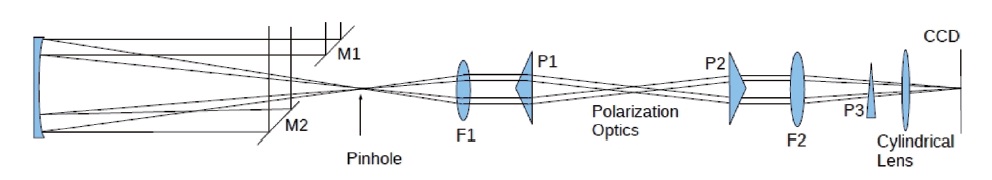
Spatial filtering minimizes the effects of rapid atmo-spheric amplitude and phase errors. The spatial filter at the input of a beam combiner can either be a pinhole or “polarization preserving” optical fibers.
This generation of optical interferometers (and pos-sibly the next) employs mirror trains which introduce instrumental polarization that can be much larger than the polarization of an astrophysical source (Elias 2001, 2004a), perhaps up to 10%. To minimize common-mode (classical, arm-based) and differential (interferometer, baseline-based) instrumental polarization, the beam combiner should use mostly refractive optics with as few reflective optics as possible or employ orthogonal pairs of reflective optics. For easier alignment, we choose the former.
Calibration will be simplified if no instrumental polar-ization is introduced after the polarimeter within a beam combiner. In general, instrumental polarization depends on telescope pointing. Counteracting this effect with spe-cialized optics has been demonstrated by Rousselet-Per-raut et al. (2006), but we assume instead that a polariza-tion calibration model of the complete instrument will be created and maintained.
Like amplitude errors, random differential atmospher-ic phase errors occur at relatively high frequencies. They can be minimized by coherent averaging and phase boot-strapping in conjunction with closure phases (Armstrong et al. 1998, Jorgensen et al. 2007). Coherent averaging re-quires measurements at multiple wavelengths, and this has been demonstrated with Navy Prototype Optical In-terferometer data.
Dispersing the fringes on a low-read-noise charge-coupled device is a logical choice for coherent averaging. Phase boot-strapping requires simultaneous measure-ments using non-polarimeter channels (same wave-lengths as the science channels) on multiple baselines (some must be relatively short). Existing interferometers and their fringe trackers can accommodate this require-ment (and also provide photometric normalization, if necessary). Slowly changing instrumental phase errors can be removed as part of imaging processing.
Taking these requirements into account, we created a preliminary spectrally dispersed image-plane polariza-tion beam combiner (Fig. 3). The only reflecting optics used in the entire design feed the instrument. Different polarimeter configurations can be substituted as desired. This beam combiner is designed for sequential measure-ments of a single baseline. The spectral resolution can be changed with different wedges, and the design can be ex-panded for simultaneous measurements and/or multiple baselines.
We are also in the process of designing a beam combin-er with simultaneous measurements of all polarimeter states. For each telescope input, it splits the light into or-thogonal linear components and sends the light through fiber spatial filters. The beams are then combined to pro-
duce all of the zero-spacing and interferometric correla-tions that are eventually transformed into Stokes param-eters.
4. PRELIMINARY POLARIMETER DESIGN
For a simultaneous beam combiner, the polarimeter is built in. The light from each telescope is split into two orthogonal states immediately before interference. These optics cannot be easily replaced. For a sequential beam combiner (Fig. 3), however, the polarizing optics can be replaced as desired. In this section, I will discuss only the polarimeter for the sequential beam combiner in the pre-vious section.
We have a choice of using a separate polarimeter for each arm or a single polarimeter placed after beam com-bination. The single-polarimeter design simplifies instru-ment design as well as calibration, so we will employ it in the preliminary design. The polarimeter should be able to measure all Stokes parameters, not only for astrophysical use cases but to provide the best instrumental polariza-tion calibration.
Beam combining optics must be as stable as possible to improve calibration, which means minimizing mechani-cal and thermal disturbances. A rotating linear polarizer introduces vibrations, so we will not use it. In addition, all polarizers possess a small optical wedge which causes the beam to wander on the detector when rotated, thus com-plicating calibration. To vary the polarimeter state, we will use liquid crystal (LC) retarders that apply no wedges and minimal heat.
As mentioned in the previous section, atmospheric amplitude errors occur at relatively high frequencies. They are produced by scintillation and variable extinc-tion. The instrument must be able to normalize these effects.
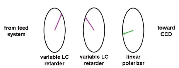
Fig. 4 is a schematic representation of a polarimeter employing two variable LC retarders (one-wavelength range) and a fixed linear polarizer. Varying the voltage on the retarders changes the polarimeter state. Research is being performed to determine the optimum orientations, modulation patterns, and timings. Multi-output linear polarizers, such as a Wollaston, are also being considered to replace the single-output linear polarizer.
5. END-TO-END OIP DATA REDUCTION
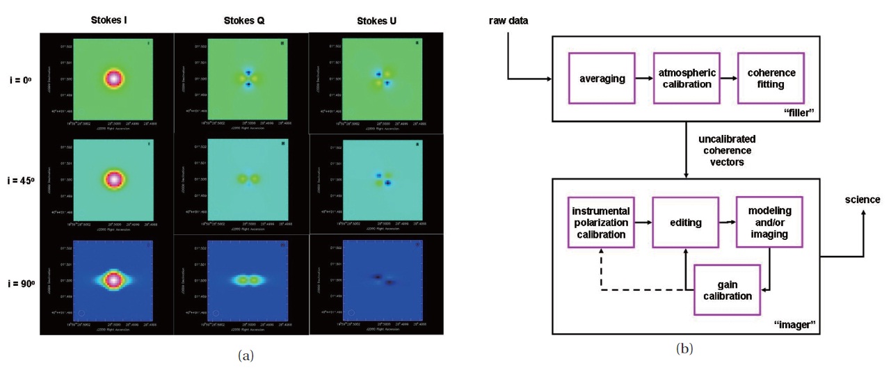
We have created 2.2 ㎛ Be star models (Mackay et al. 2009). We imported them into CASA, turned them into noiseless one-second visibility samples for a scaled 27 telescope VLA-like array, and reimaged them (Elias et al. 2011). All Stokes images showed the disk, although it was
easier to see in the Stokes Q and U images because the bright and unresolved star is unpolarized.
We have recently implemented more realistic simula-tions, employing: 1) 9 antennas in a “Y”; 2) 15 channels from 2.1 to 2.5 ㎛; 3) Poisson noise; and 4) random phase errors, standard deviation of 10?. The star is B0Ve at a dis-tance of ~60 pc, which means that the Johnson V magni-tude is ~0. The maximum baseline is longer than existing interferometers, ~1,500 m, but simulations with baselines a factor of few smaller still show the polarizing structures. Also, baselines at optical wavelengths are a factor of ~3 smaller. These two factors together set the maximum baseline well within the limits of existing interferometers and allow observations of smaller objects.
In Fig. 5b, we present a preliminary top-level design for end-to-end OIP data reduction. We will systematically write and test the software as part of a future study. The images of Fig. 5b were created as part of the imaging box in Fig. 5a.
Raw data (~millisecond samples), including errors, will eventually be created from the Be star models. The raw data will be written to uvfits or OI-FITS files, which are used for optical interferometry data. The filler, which has not yet been written, processes the raw data into ~ one-second uncalibrated coherence vectors and writes them into a measurement set (MS), the native CASA data for-mat. At present, there is special software to convert the Be star model files directly to MSes with one-second aver-ages without forming raw data.
The polarization calibration observation strategy may take a number of forms. For example, an instrument mod-el, including variability caused by pointing, can be fitted to observations of polarization calibrators. The model is maintained independently of science observations. Or, one may perform observations of polarization calibrators near the science targets (in both time and location on the sky). The instrumental polarization is then assumed to be ~the same for both source types. Regardless of strategy, the polarization calibration data must be converted to a form that the native CASA task polcal can use. This con-version software does not yet exist, and it will probably be written in the CASA environment.
CASA already possesses mature visibility viewing and editing tasks such as msview and plotms. It also has an advanced imaging task called clean. It may be configured for multifrequency synthesis, which is relevant for most optical interferometry data because they typically are obtained over wide wavelength ranges. Multiscale clean, which uses arbitrarily shaped components (as opposed to a simple delta function), is also available.
Steady progress has been made in the OIP field dur-ing the last decade, including algorithm development (Geisler et al. 2008), system engineering studies (Elias et al. 2004a,c), and hardware (Stee et al. 2006). Because of this progress and our hardware and software designs, we are confident that full-Stokes imaging with optical inter-ferometers will become commonplace in the near future and provide new insights into many astrophysical objects and phenomena.