A binary star story of some years hence might begin: “ once upon a time there was a model feature that needed further work (UD for under-developed), and another that could have been applied but was not (UU for under-utilized). UD was not dressed for the science scene and UU was all dressed up with no place to go.” We have experienced both situations in the early growing pains of high definition television and 3D TV, where few promoters were covering production costs for lack of in-home receivers (UD) and few persons bought receivers for lack of on-air productions (UU)-an iterative loop with very slow convergence at start-up. So development and utilization can interact, as in the modeling and analysis capabilities now to be discussed. Many of these model features are covered with considerable detail, with further references, in the book by Kallrath & Milone (2009).

An observational pursuit in need of analytic progress is growth and decay (briefly aging) of magnetic starspots for tests of theoretical work on outer convection zones and their dynamos. A realistic aim is to establish the statistics of spot (and spot group) area versus time over ranges of star mass, composition, envelope rotation, and age, without attempts to assess configurational details. Many parameters compete for attention, so spot temperature variation can be disregarded to reduce the parameter count, given that magnetic spots are nearly black in the first approximation. Eclipsing binaries (EBs), ellipsoidal variables, and rotating single stars can be targets. The literature on observed star spots is rather large so only some examples can be given. Tomography of spectra gives excellent results, as in Vogt et al. (1987), Hatzes (1998), Richards et al. (2010), although light curve data are much more abundant and usually easier to obtain. Distribution and/or aging of spots based on light or radial velocity (RV) curves has been examined, for example, by Kang & Wilson (1989), Pettersen et al. (1992), Hall (1994), Hall & Henry (1994), Rodono & Cutispoto (1994), Helminiak & Konacki (2011), Helminiak et al. (2011). Sunspots, being spatially resolved and regularly monitored, need only statistical (not light curve) analysis and are an obvious information source, although only for one star. The part of the sunspot literature that bears most directly on this paper is spot aging, for which graphical and digital data as well as fitted formulas and theory can be found, for example, in Howard (1992), Wilson (1984), Petrovay & van Driel-Gesztelyi (1997), Solanki (2003), Livadiotis & Moussas (2007), Hathaway (2010). Sunspots show a wide variety of growth and decay forms, yet are not likely to close the book on spot aging. Another potential application is to accretion hot spots, where major excursions in spot area and temperature can be expected in response to stream variations in flow rate and trajectory.

The effective spatial resolution for light curve based spot observations is limited, as it comes not explicitly but from multi-aspect views of eclipses of a rotating surface via what might be called photometric tomography. Several binary star light curve models have included spots (see Wilson [1994] for background and historical references), with limited geometric precision. For example, the Wilson & Devinney (WD) model (Wilson & Devinney 1971, Wilson 1979, 1990, 2008) previously considered each surface element to be entirely in or entirely out of a given spot, based on location of the element’s center. A major precision improvement due to partial area assessments is outlined below. Good starting parameter estimates are needed in regard to spot motion (surface rotation and drift) as well as location and size at a reference time. Nearly continuous light curve runs now come from advanced instrumentation such as the Kepler mission, from surveys such as optical gravitational lensing experiment (OGLE) and all sky automated survey (ASAS), and from ground-based automated telescopes.

Advances are in order if the remarkable precision of Kepler mission light curves is to be fully exploited. Those discussed here are:

2.1.1 Refinement of Spot Specification for Size and Motion

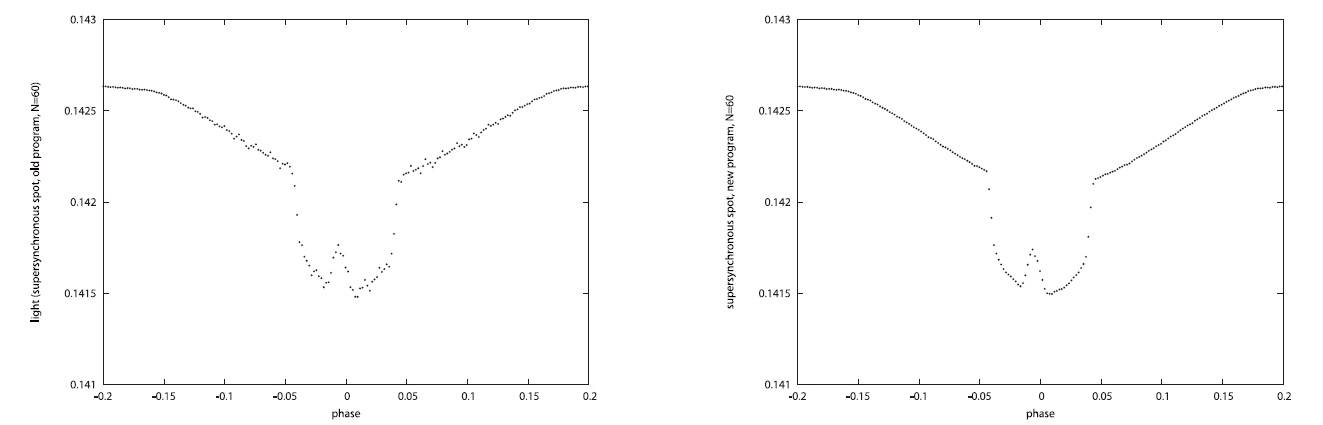
Numerical noise can be greatly reduced via fractional in-spot area assignments for surface elements. The limited spatial resolution of light curves precludes meaningful refinement of spot shapes (giraffes are not to be found) but computational noise due to spot size change and motion can be reduced. A model that specifies spots and surface elements via position vectors now is operational and will appear in Wilson (2012).

2.1.2 Simple but Informative Growth-Decay Curves

A useful spot aging model needs a non-constraining waveform and individual spot development. The waveform should have only a few parameters so as to maintain simplicity. Such features allow expression of spot aging essentials without imposition of pre-conceived ideas. For now the waveform starts from zero spot area, rises linearly to a pre-maximum, continues at constant level to a post-maximum, and declines linearly to zero area at disappearance. The aging model can be revised in the light of experience. Growth-decay parameters are maximum spot radius and four moments in time -onset, pre-maximum, post-maximum, and disappearance.

Magnetic spots can drift with respect to the rotating surface and the surface may rotate asynchronously relative to the orbital motion. Computational precision becomes especially important for asynchronous motions because model spots then move with respect to the surface elements, thus making each momentary configuration a separate numerical problem (as opposed to overall star rotations). The multiple spot-element registrations then change continuously with binary phase and have potentially serious consequences for small amplitude variations, where computational noise could exceed observational noise. The situation can be troublesome for spots that might be mistaken for transiting exoplanets.

An outline for vector treatment of spots can begin with specification of a polygonal surface element by a position vector for each vertex and some small number of uniformly spaced position vectors along each side. With, say, three interpolated vectors and the two vertex vectors there will be five vectors per side. Now assign another position vector to the spot center and, by spherical trigonometry and iterative vector operations, either locate the spot rim’s intersection with the element side or determine that there is no intersection. With all spot-element intersections thus determined and the element broken into triangles, areas of the in-spot and out-of-spot parts of each element can now be calculated with the triangle and circle area formulas of spherical trigonometry, although the various intersection cases must be treated separately. Mathematical details are in Wilson (2012). Each spot’s overall temperature factor (T-factor = ratio of mean element temperature to local unspotted temperature) is an area-weighted mean of the out-of-spot T-factor (unity) and the in-spot T-factor (an input quantity).

Simulation solutions are underway for recovery of spot parameters, to be followed by similar solutions for real stars.

Spectral line profiles have been in the WD model for about 20 years, with inclusion of all ordinary binary system effects such as eclipses, rotation, tides, gravity brightening, reflection, and so on. The profiles are computed rather rigorously, in so far as those effects and line blending are concerned. A likely reason for the facility’s lack of use is that moderately high resolution spectra are needed for meaningful applications, although the required spectrographs certainly exist. Intrinsic broadening (damping, thermal Doppler, turbulence, etc.) can be added if there is interest. Potential useful output is connected with each physical effect. EB’s give added stellar atmosphere information via line profiles, vis ? vis single stars, for the same reasons that apply to light curves. Simultaneous solutions with other data types could be optional, would ensure coherent results, and may be the main benefit. With stellar atmosphere parameters added to binary star parameters, the list may seem excessively long but, as always, not all have to be evaluated at once.

The usual EB ephemeris data are eclipse timings. A frequently encountered situation is to have many such timings but no more than one epoch of full light curves or RV curves, so most or all of the ephemeris information is in timings. In other circumstances, typical of recent discoveries from large scale surveys, there are good light curves over extended intervals or at multiple epochs, perhaps supplemented by RVs, with few eclipse timings beyond those in the full light curves. Although RV curves usually lack sharp features to serve as timing ticks, they do carry timing information and can fill gaps in light curve records.

An alternative to ephemerides from eclipse timings is ephemerides from whole curves (Hadrava 1990, 2004, Elias et al. 1997, Wilson 2005, Van Hamme & Wilson 2007, Mikulasek et al. 2011). Relations for conversion of time interval to phase interval are in Wilson (2005) (including series approximations needed when dP/dt is close to zero) and in Kallrath & Milone (2009). An advantage of generalized simultaneous solutions with embedded ephemeris parameters is that apsidal motion (i.e. orbit rotation), third body reflex kinematics, and rate of period change (dP/dt) as well as other EB parameters, can interact with the period and reference time when all observations are utilized. Whole curve ephemeris solutions have been in the WD program since 1998 and applications have begun to appear (Van Hamme et al. 2001, Williamon et al. 2005, Van Hamme & Wilson 2007, Wilson & Van Hamme 2009, Wilson et al. 2009, 2010, Wronka et al. 2010, Wilson & Raichur 2011). The Mikulasek et al. (2011) contribution explicitly adopts a template to represent a phased light curve that can pertain to any kind of periodic variable star. The other contributions are designed to work within a general EB solution program, although they could be applied to other types of variable stars if a variation model or template were added. The embedded schemes are basically template-sliding (implicit or explicit). The template in the WD model is the iterated theoretical light/velocity curve, or actually curves in multiple bands. In a sense the process can be described as template-free, as the various curves need not be the same from cycle to cycle but can develop over time, as in the case of stars with magnetic spots.

One should go where the observations are. Accordingly both whole curves and timings can be entered together in solutions for the usual ephemeris, as well as apsidal motion and third body orbital parameters. No conceptual difficulties stand in the way - practical realization awaits only programming, testing, and documentation. The resulting program will apply to light curves, RV curves, and eclipse timings in any combination. The usual conscientious attention to weighting will be needed.

Attenuation by circumstellar matter has been in the WD model for more than 10 years, with two kinds of wavelength-dependent absorption as well as electron scattering. Wavelength-dependence is by a power law and also has extra components that represent line absorption averaged over each photometric band. The scattering material is in spherical clouds at fixed locations in the system’s rotating frame. The clouds could be made to move by adding an orbit integrator if there were potentially important applications, so as to investigate moving structures. Attenuation along the line of sight to each surface element of each star is computed, and results are combined for any line of sight that passes through more than one cloud. So far the circumstellar matter feature has been applied only to AX Mon (Elias et al. 1997), which seems to have a stationary accumulation of material where a mass transfer stream self-intersects after having passed around the hotter star.

Absolute EB light curves in the Johnson, Cousins, and Str?mgren bands, together with RV curves, now can be solved effectively for distance and both star temperatures, given flux calibrations by Johnson (1965, 1966), Bessell (1979), Fabregat & Reig (1996), Gray (1998), Wilson et al. (2010). Implementation is in a recent version of the WD program¹. Although non-absolute light curves yield only a temperature relation,T₂ = f (T1₎, several points favor absolute light curves as providers of definite temperatures. The overall situation is discussed at length in Wilson (2008) and in Wilson & Van Hamme (2010), and can be briefly summarized in the temperature-distance (T - d) theorem, which says thatT₁, T₂, and d can be found from RV’s and a minimum of two absolute light curves (in substantially different photometric bands). Results have been published for V505 Persei and WZ Ophiuchi by (Wilson et al. 2010) and for ER Vulpeculae, V1143 Cygni, and ε Coronae Australis by Wilson & Raichur (2011). Distances agree well with parallax distances from the Hipparcos mission (Perryman et al. 1997, van Leeuwen 2007). Until recently there was much difficulty in placing light curves on standard photometric systems due to lack of standard magnitudes for comparison stars, but that problem has largely disappeared due to publication of standard magnitudes by Landolt (1992, 2007, 2009) and others. Accordingly, solutions for photometric temperatures and distances are soon likely to appear in quantity.

1To retrieve the 2010 version of WD, go to anonymous FTP site ftp.astro.ufl.edu, change to sub-directory pub/wilson/lcdc2010/, and download all the files.

The long-recognized light time effect due to a binary system’s motion about a triple system center of mass can improve multiple star statistics, with help from corresponding RV shifts. The phenomenon is well known from eclipse timings and its analysis from whole light and RV curves has begun (Hadrava 1990, 2004, Van Hamme & Wilson 2007) (VW). A brief summary of recent history is in VW, where the relative importance of light-time and RV input is assessed. Combined light and RV data give better temporal coverage than either type alone so as to reduce difficulties due to gaps in the observational record. Naturally solutions from mixed data types require conscientious attention to weighting if light and velocity information is to be properly balanced. However overall human workloads are reduced because the entire theory is within the computer model, so results are generated impersonally with only minimal subjective judgment. VW found whole curve solutions to give comparatively small standard errors, vis ? vis eclipse timings, in reference epoch, period, and rate of period change for DM Persei over roughly the same time span. Time-wise gaps have been a very serious impediment to third body kinematic work, but extended coverage from surveys such as Kepler and ASAS should give new freedom from the gap problem. Gaps lead to the common problem whereby genuine and aliased periodicities are difficult to distinguish. Even if an assumed period is correct, there are correlations among third body reflex motion, period changes due to mass transfer, and apsidal motion, so we definitely do not want aliasing problems also. In the presence of serious gaps, period sifting by power spectral analysis and cleaning algorithms is indispensable in preliminary work. As in § 4, entry of eclipse timings with whole light and RV curves can fill gaps in the time-wise baseline or extend it.

Substantial effort has gone into polarization surveys. However a focus on variability of individual objects, particularly close binaries, could stimulate a burst of activity on analytic models. Some polarization phenomena are periodic, some not, so polarization data need to be documented with observation times², which has only sometimes happened in past publications, rather than fractions of a cycle (i.e. phases). A common publication practice for polarization is phased data in graphs without digital tabulation, thereby explaining the scarcity of binary polarization models. There are very good papers on computations relevant to polarization mechanisms, e.g. Brown et al. (1978), but little on complete models that combine polarization with other close binary phenomena. Most published computations are attempts to fit corrected observations, analogous to the rectified light curves of 40 years ago. Published analyses often involve the unnecessary step of fitting by Fourier series, which requires judgments of how many Fourier terms to include and undermines proper computation of standard errors. A useful form of publication would consist of Stokes quantities or the equivalent polar angles and magnitudes vs. time.

A model that avoids these shortcomings is that of Wilson & Liou (1993), which could be developed further if a reasonable amount of EB polarization curve data existed, particularly for Algol type binaries. The theory is built upon a physical binary star model with all the ordinary effects such as tidal and rotational distortion, gravity brightening,

[Fig. 1.] The panels show a synthesized eclipse as a planet transits a star, with an upward spike where a dark spot is covered. The visible noise is caused by spot motion with respect to the surface grid. Ordinarily the computational noise would not be noticeable, but here the flux drops by only a half-percent in eclipse, so the vertical scale is greatly stretched. The left panel was computed with the public Wilson & Devinney program and the much smoother right panel with a developmental version with surface elements that can be partly within a spot (position vector treatment).

reflection, etc. Limb and circumstellar polarization due to electron scattering are included, with no attempt to remove effects from the observations. Observable Stokes quantities are synthesized by combining the limb and circumstellar polarizations, with attention to sign conventions and handedness of coordinate systems. The model avoids the common simplification that all photospheric polarization is generated in a thin ring at the limb, thereby attaining considerable accuracy improvement. Finally a solution of the observed data by the method of differential corrections gives parameter values that characterize the circumstellar matter distribution and photosphere, with standard errors. The model is rigorous in its internal operations but needs some astrophysical refinements.

2See Hoffman et al. (1998) for an example of properly tabulated polarization data.

Sunspot-like starspots and accretion hot spots can now be modeled with greatly improved precision and with timewise variability as well as motion. The required observations can come from the Kepler mission and other surveys, with those from Kepler being very precise. Accordingly, improved precision of the spot model is not a mere nicety but may be urgently needed, especially for exoplanet applications where an eclipse depth may be very small and spots can temporarily be mis-identified as planetary transits. Close binary ephemerides from whole light and RV curves now complement those from eclipse timings and are beginning to have increased application. Reflex motion of binaries due to third bodies need not be treated separately from other parameters but can be analyzed within a general light/RV curve solution. Attenuation by circumstellar matter can also be so handled. Motions of circumstellar clouds and streams remains untreated but could be added if there are potential applications. EB solutions in absolute flux now find distance and two star temperatures in one step, while reducing subjective decision making to a minimum and avoiding all spherical star approximations. Broadened and blended spectral lines are in the WD model. Damping, thermal Doppler, and other broadening mechanisms could be added if the necessary high resolution spectra exist. A similar situation attends binary star polarization, where published polarization curves could encourage modeling advances.