The BINSYN program package is based on an earlier program that simulated classical binary star systems. That program included a light synthesis procedure described in Linnell (1984) and an extension to include differentials corrections in Linnell (1989). A spectrum synthesis capability for classical binary stars was added in Linnell & Hubeny (1994) and the capability to simulate the spectra of binary stars with an optically thick accretion disk was added in Linnell & Hubeny (1996). Beginning with that extension the name BINSYN has been used in connection with the program package.
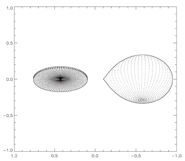
The primary application of the spectrum synthesis capability has been analysis of cataclysmic variables (Linnell et al. 2008a, b, 2010a, b, Szkody et al. 2008). See Fig. 1 for a BINSYN projection view of a cataclysmic variable.
Until 2009 BINSYN ran on a PC using Windows as an operating system. In 2009 a migration began to a Linux system. The spectrum synthesis capabilities that had been developed prior to 2009 were unrelated to the original study of eclipsing binary (EB) light curves; the EB procedure, dormant during the study of cataclysmic variables, used a black body representation of the stellar radiation characteristics.
The Linux version of the complete package evolved to become very different from the Windows version. A plan
developed to release a public version of BINSYN; this plan required consideration of a procedure for EB light curve solutions that was more realistic than the black body approximation. This report describes the present status of that effort.
The BINSYN capability to produce synthetic spectra specific to a particular binary star system, including compositional anomalies, invited consideration of a synthetic photometry approach. If successful, the approach would provide both synthetic spectra and synthetic light curves. Analysis of light curves produced with new or unusual color filters could be accomplished with simple substitution of filter response calibrations for the particular photometric system.
The current version of BINSYN appears to be the only available program package that simulates both classical binary star systems and those that include an optically thick accretion disk. (By “ simulates” we mean starting with
The basic plan of BINSYN is to divide the entire simulation into program segments with each segment comprising a separate program. The program segments then are linked together by a procedure described below. For example, the calculation of a model to represent the 3D geometric shape of the individual stellar components, including a grid that defines their shapes, is performed in a program called PGA. That program uses a gravitational potential, in physical units, to define the photospheres. A separate (prior) program, CALPT, supplies those data for the Roche model (this arrangement provides an alternative for a different future model, say a polytrope model). A succeeding program, PGB, provides orbital parameters: inclination, eccentricity, longitude of periastron, and one or more orbital longitudes. It calculates the projections of the photospheric grids on the plane of the sky, determines the horizon points for the photospheric grids, and determines visibility keys for grid nodes (intersections of longitude and colatitude contours): with three options: either visible, below the observer’s horizon, or eclipsed. Next, program PGC determines radiation characteristics of the components.
PGC input data include the polar
The following program, PGD, calculates the light intensity in the observer’s direction in each of the specified observation wavelengths; it also evaluates the light lost by eclipse in the separate observation wavelengths. A separate program, RDVEL2, determines the component radial velocities (relative to the observer) of each grid node and produces a radial velocity curve separately for the system components.
At this stage the component radiation characteristics are represented by black bodies at the local
The revised BINSYN continues to a synthetic photometry calculation of light curves; this step requires system synthetic spectra at the orbital longitudes specified by program segment PGB.
A separate program, ACPGF6, serves as an interface to an external set of model atmosphere synthetic spectra and produces a system synthetic spectrum as well as a separate synthetic spectrum for each stellar component. Note specifically that the external model atmosphere synthetic spectra must be supplied from some source such as the grid of Kurucz synthetic spectra or calculated from. e.g., the Hubeny program SYNSPEC. Finally, program SYNPHOT convolves each system synthetic spectrum with separate filter transmission curves to produce a simulated observation set (e.g., UBVRI) at the individual orbital longitudes.
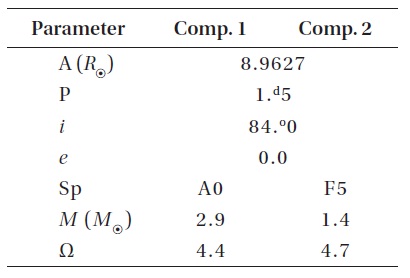
We illustrate the present status of the development effort with a test case: Parameters for it are in Table 1. Detailed parameters calculated for the components are in Table 2. As
[Table 1.] Distances are in solar radii; masses are in solar masses, Ω1 and Ω2 are Roche potentials.

Distances are in solar radii; masses are in solar masses, Ω1 and Ω2 are Roche potentials.
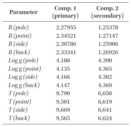
Distances are in solar radii; masses are in solar masses; temperatures are Teff values in Kelvins.
an illustration this paper includes a differentials correction solution of a synthetic light curve set (UBVRI) based on the Table 2 parameters.
Each program (segment) resides in a separate directory. Each directory includes a script that runs the program (e.g., the script in directory PGA is named pga, and is run by the Linux command ./pga), using data files that reside in that directory. BINSYN also provides a separate input data directory, named IA, for use by all programs, and a general purpose output data directory named OA. Each separate program directory (e.g., PGA) includes a script, separate from the one that simply runs the program (i.e., ./pga), that first copies necessary input data from IA to the local program directory, then runs the program, and then copies the local directory output data to directory OA. In the case of PGA, the latter script is called pgascr and is run with the Linux command ./pgascr.
Information to model a particular binary system resides in a separate appropriately named directory, with the name assigned by the user. That directory contains copies of all input files needed for a complete simulation; the required set of files can be copied from an existing directory for a different system and the parameters then initialized for the system under study. A master control script in the new binary system directory then copies all of the necessary input files (initialized as just described) to directory IA and successively commands the separate programs to run in sequence. The command to run a given program activates the script in that program directory that copies input files from IA, runs the program, and copies output files to OA. At the end of the sequence of run commands applied to separate programs, the master control script copies important output files from OA to the local system directory for examination by the user.
The list of programs to be run is much longer than the short list of programs named in the previous section and may include the sequence for a differentials correction optimization.
The advantage of the layers of scripts is that the user need not leave the directory for the system under study; he/she simply waits for completion of the run under control of the master control script and examines the output. There may be more than one master control script in the system directory. For example, it may be desirable to run separate black body and synthetic photometry simulations.
As described above, the analysis simulates the actual observational procedure with synthetic photometry. Basic references regarding synthetic photometry are Bessell (1990) and Bessell et al. (1998). We have tabulated the UBVRI filter response curves using the most recent calibration data (Bessell 1990 and private communication) to convolve with the calculated synthetic spectra.
Linnell (1989) describes the synthetic photometry procedure; the program produces a separate U, B, V, R, and I photometric "measurement" at each of the specified orbital longitudes. For synthetic photometry it is important to use continuum synthetic spectra rather than line spectra; the changing Doppler shifts of the line spectra with orbital motion cause very small but undesirable photometric modulation when convolving the spectra with the filter transmission profiles.
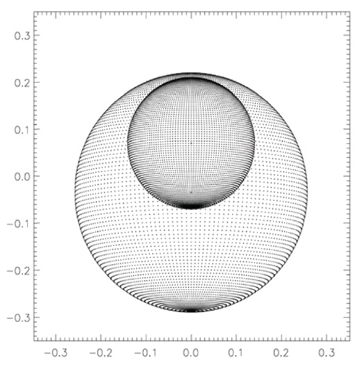
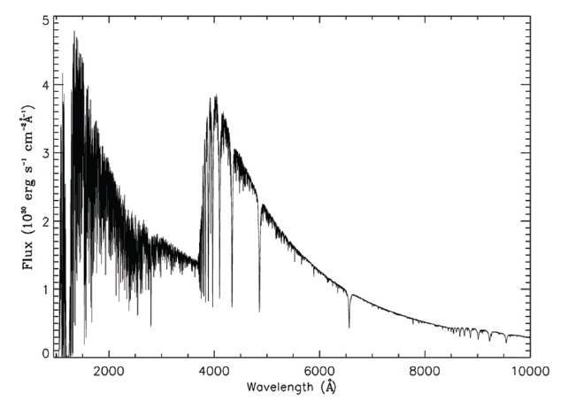
In the current example there were 101 orbital longitudes. An accurate and smooth theoretical light curve requires a fine photospheric grid; this example used 91 colatitude profiles and 151 longitude divisions. A projection view of the system at orbital longitude 0.0 is in Fig. 2. A sample synthetic line spectrum at orbital longitude 0.0 is in Fig. 3 (we
do not show the corresponding continuum spectrum).
Using the basic U, B, V, R, I light curves described above, separate programs produce a denser grid of points by interpolation and modulate them with random noise of specified standard deviation (0.0001 in the current case) in each separate color light curve.
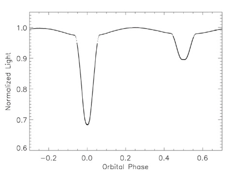
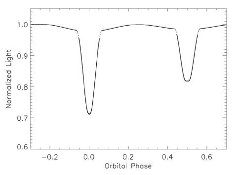
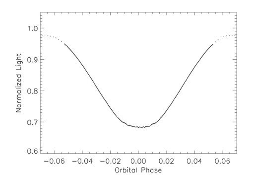
These become the "observed" light curves. We then displace one or more of the system parameters and seek a differentials correction solution as a test of the solution technique. The U light curve is in Fig. 4 and the corresponding I light curve is in Fig. 5; the theoretical light curves are superposed in each case. The B, V, and R light
curves (not shown) lie between the extremes of Fig. 4 and Fig. 5. The model parameters used for determining first, second, etc., contacts inadvertently differed slightly from the values actually used in calculating the light curves: this explains the short sections showing only the reference data values. Fig. 6 shows the central part of primary minimum in detail. Note the slight irregularity of the light curve: this arises from the "granularity" of the photospheric grid and limits the achievable accuracy of the solution. The word "granularity" means that the visibility key for a given photospheric segment either includes the entire segment or excludes it from the summation process; a future development will determine fractions of a given segment to include.
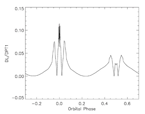
The solution procedure is the same as described in Linnell (1989). Partial derivatives of system light with respect to the various system parameters are required as function of orbital phase. A separate set of programs adopts central reference values of system parameters and, for each parameter, a value displaced above the central reference value and a value displaced below the central reference value by an equal amount. These programs then calculate light curves for all three parameter values, tabulate the first differences and then the second differences as function of
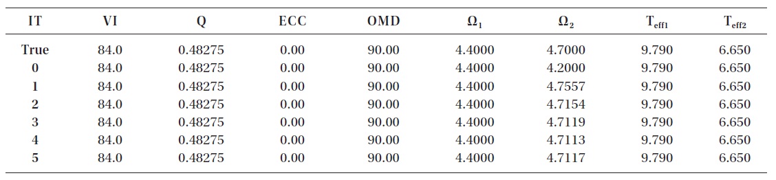
The optimized parameter is Ω2 in column 7. The first line lists the true value, the second line lists the assumed value. Successive lines list results of successive iterations.
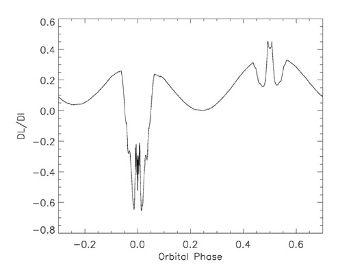
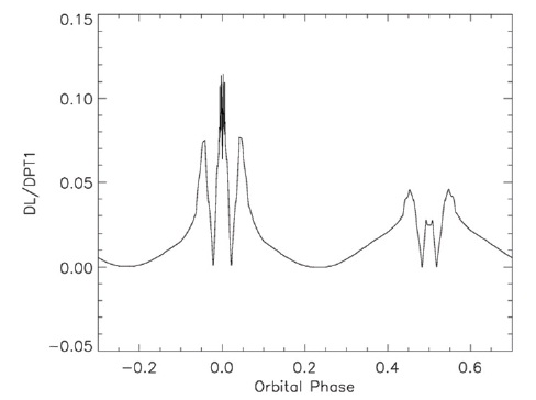
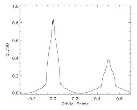
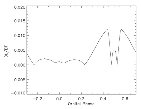
orbital phase. Finally, the programs use Stirling interpolation to calculate the required derivatives. See Linnell (1989) for details. Illustrations of the partial derivatives are in Figs. 7-12. Since the orbit has zero eccentricity there is no partial derivative with respect to orbital eccentricity or with respect to ascending node.
As a test of the solution program, we start with a single incorrect system parameter, Ω2. Table 3 tabulates the solution. The first line of data lists the true values of the parameters appearing in the column headings. The one incorrect parameter value appears in the second data line (identified in the first column as data line 0). Successive iterations appear on successive data lines. The software
inserts these data lines automatically during the iterative solution.
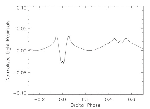
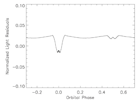
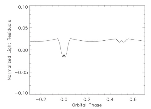
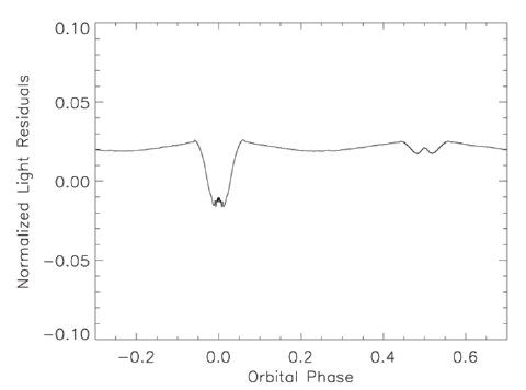
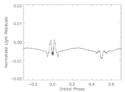
The U residuals from the initial approximation are in Fig. 13. The residuals after the first iteration are in Fig. 14. There are corresponding residuals for the other colors; we show only the U residuals. The residuals after the second iteration are in Fig. 15; Fig. 16 shows the residuals after the third iteration. There is little improvement after the third iteration; Fig. 17 shows the residuals after the fifth iteration. Note the displacement of the outside-eclipse residuals from an average value of 0.0; this indicates a residual program bug. The running time per iteration is approximately 55 minutes and is a strong function of the fineness ("granularity") of the
photospheric grid. The accuracy achieved for the parameter subject to optimization, Ω2, is 0.25%. Provided tests with combinations of optimized parameters produce comparable results, this accuracy is adequate for analysis of high quality ground-based photometry.
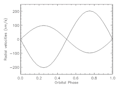
A separate objective may be to produce a synthetic spectrum at a particular orbital phase for comparison with an observed spectrum. In that case the externally-referenced spectra must be line spectra. A different (simpler) master control script accomplishes that objective without performing a differentials correction. An example of the use of BINSYN to model a binary system spectrum is in Linnell et al. (2006). The radial velocity curves for the current example are in Fig. 18.
The basic reference for analysis of accretion disk systems is Linnell & Hubeny (1996). Inclusion of the accretion disk adds two objects, the accretion disk face and rim, to the original list of objects to be modeled. A concentric series of annuli represents the accretion disk. Inclusion of the two additional objects requires addition of a series of programs that parallels the treatment of binary stars. Moreover, this addition requires inclusion of the new programs in the differentials correction solution sequence (master control script) described above for classical binary stars. In the case of a classical binary star without an accretion disk, the accretion disk routines do not actually run but their control information must be read to specify that no accretion disk is present. If an accretion disk is present the data file of external synthetic spectra is considerably extended since a model synthetic spectrum must be supplied for each accretion disk annulus as well as one or more synthetic spectra for the accretion disk rim. The accretion disk routines include a capability to model a rim hot spot.
The BINSYN program suite has been ported from a Windows operating system to a Linux system. The original capability to perform differentials correction parameter optimization using black body representation of component radiation characteristics has been preserved, together with capability to represent stellar components and an accretion disk with synthetic spectra. Based on the experimental results reported here, the differentials correction procedure for EB light curve solutions using synthetic photometry works correctly although one or more bugs remain to be removed. Further experimentation is required to validate BINSYN for combinations of parameters.