The sunspot number provides the longest available record of solar activity. Although its short-term variations give some important insight, e.g. regarding solar differential rotation, its long-term behavior and the longevity of its series may provide many more such insights. This is why the international scientific community has continuously renewed its interest in the sunspot number. Many scientific investigations, including cycle analysis and forecast, solar North-South asymmetry analysis, coherence analysis of the solar magnetic field, mid-term studies of solar activity, are based on the Solar Influences Data Analysis Center (SIDC) sunspot data (Pulkkinen et al. 1999, Lockwood 2003, Solanki et al. 2004, Wang 2004, Chang 2007, Usoskin 2008, Petrovay 2010, Ternullo 2010, Kim & Chang 2011).

The SIDC (Berghmans et al. 2005) collects monthly observations from various stations worldwide in order to calculate the International Relative Sunspot Number R_i (Letfus 2000, Clette et al. 2007, Vaquero 2007). The center broadcasts the daily, monthly, and yearly sunspot numbers, with middle-range predictions (up to 12 months). The Sunspot Index Data Center was founded in 1981 to continue the work, when the Zurich Observatory decided to halt computing and publishing the sunspot number. In 1981, the Sunspot Index Data Center began producing a sunspot index, called the International Relative Sunspot Number, R_i. Continuity and coherence with the former index of Zurich was assured through the use of Locarno as a reference station. In 2000, reorganized and expanded by gaining the qualification of Regional Warning Center of the International Space Environment Service, the Sunspot Index Data Center had become the SIDC. The bulletins and reports of the SIDC are all freely available for the scientific community and the general public on the internet (http://sidc.oma.be).

In 1849, Wolf at the Zurich Observatory proposed the widely used formula: R_Z = 10g +f, where f is the number of individual sunspots, and g is the number of sunspot groups (Letfus 2000, Clette et al. 2007, Vaquero 2007). The quality factor k was introduced later in order to compare results from different observers, the stability of the Earth’s atmosphere and telescopes, giving the formula R_i = k (10g + f). Observers must satisfy several criteria to be included in the SIDC network: dedication (more than 10 observations per month), regularity (no missing months) and consistency. It is the last that is quantified through the quality factor k, which is the correction factor between the raw sunspot number of an individual station and the global network average. The correction factor k, which typically has a value between 0.4 and 1.7, ensures that results can be compared with each other. The coefficient of the reference station Locarno is fixed at the value of k_Loc = 0.6. The task of the SIDC consists of collecting the observations from as many stations as possible worldwide, determining the appropriate k factor for each of them, and extracting an overall R_i from all these observations in a good statistical sense.

Let us here briefly describe the statistical processing of input data coming from the worldwide observing network (~90 stations located in ~30 different countries). The R_i processing consists of two main steps. In the first step, the daily reduction coefficients to Locarno are calculated and monthly averaged for every station. For each station, daily values deviating by more than 2σ from the monthly station average are eliminated. The monthly averages are recomputed iteratively until k values are consistent for all stations. In the second step, using the updated monthly k coefficients, the R_i value is computed for each station, and network averages R_d and standard deviations σ are computed for each day. Elimination on the basis of a 1-sigma criterion is used on newly calculated daily means, until the number of retained stations remains unchanged, or the final relative standard deviation is lower than 10%. The final result is retained as the daily R_i. The final quality control consists essentially of regular comparisons between the sunspot number R_i on one hand, and an average of about 20 selected good stations (including the Locarno reference station) or the 10.7 cm radio flux on the other.

Recently, Oh & Chang (2012) have reported results of sunspot observations at the ButterStar observatory for 3364 days, from the 16^th of October in 2002 to the 31^st of December in 2011. By applying the linear least-squares method between the observed sunspot number (R_B) and the International Relative Sunspot Number (R_i), the overall correction factor k_b for the entire observing period was found to be 0.9519 with a standard deviation of 0.006. In addition, they attempted the same procedures in each year from 2002 to 2011. When calculated for each year, the yearly correction factor has slightly different k_b values from year to year, and furthermore shows a trend of changing along the solar cycle. That is, the yearly correction factor k_b is larger during the solar maxima and smaller during the solar minima, in general. It was then considered that it seems possible to reduce the errors in indexing sunspot numbers a little bit further by determining the correction factors year by year. Interestingly, similar conclusions were drawn by Kim et al. (2003), in which the observed data at the Korea Astronomy and Space Science Institute (KASI) were analyzed.

In this paper, we attempt to tackle the question of whether the variation in the correction factor is really coupled with the solar cycle . We also investigate the question of whether this apparent dependency is due to a possibility of lower statistical confidence in the linear least-squares method with a decreasing number of sunspots. If the apparent dependency is indeed due to an artifact in the statistical treatment, researchers should refrain from correcting the observed sunspot numbers R_B on a yearly basis, even though it seems to result in a better agreement. This paper is organized as follows. In Section 2, we briefly introduce the artificial data set used in the present analysis. The results we have obtained are presented in Section 3. Finally, we discuss our results and make some conclusions in Section 4.

We model the sunspot number with random noise superposed on a slowly varying background to characterize the sunspot numbers, as per Chang (2008). The underlying part of the sunspot number data is assumed to represent a sum of undamped oscillators. Thus, the international relative sunspot number R_i is assumed to be approximated by

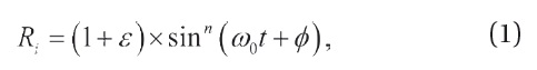
where ω₀ represents the solar cycle frequency, ? is the phase shift, and ε is random noise. The value of n can be chosen arbitrarily as long as the resulting function resembles the observed sunspot number data. Throughout the paper, ω₀ corresponds to 11 years. We employ two kinds of noise distributions for ε in the current paper: 1) uniform distribution, with which random numbers are distributed uniformly between 0 and 1, and 2) exponential distribution with a unit mean and deviation. It is observed that the multiplicative random noise reproduces observational features more satisfactorily (Chang 2008). This is why we adopt the multiplicative random noise rather than the additive random noise.

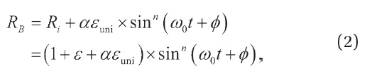
To simulate calculating the correction factor k, we need to generate a time series of the observed sunspot number R_B given by

where ε_uni represents the random error which is assumed to obey the uniform distribution between 0 and 1, and α is a measure of signal-to-noise ratio. Other symbols have the same meanings as in Eq. (1). We consider ε_uni occurs due to different degrees of the skill of various observers, the atmospheric stability of the observing site, the capacity of telescopes, and so on. One may also consider α as

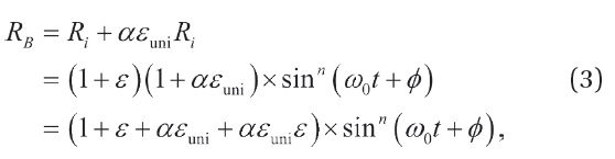
whose only difference is the negligible term, αε_uniε. We take this particular form of multiplicative noise since it agrees with the observed features quite well (Chang 2008). That is, in the period with a large number of sunspots, uncertainties are relatively large due to the large number of sunspots.

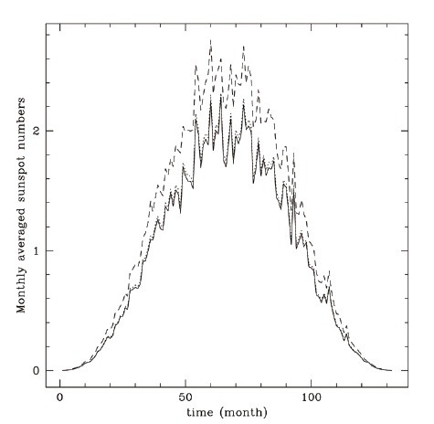
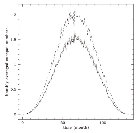
In Fig. 1, we show the monthly average of modeled sunspot numbers generated with the exponentially distributed random noise, ε, as a function of time in a month. The abscissa is time in months elapsed since a solar cycle begins, and the ordinate is measured in an arbitrary unit. The solid line represents R_i generated by Eq. (1). The dotted and the dashed lines correspond to R_B generated by Eq. (2) with α = 0.1 and α = 1.0, respectively. In Fig. 2, similarly, we show the monthly average of sunspot numbers generated with the uniformly distributed random noise, ε. The solid line represents R_i generated by Eq. (1). The dotted and the dashed lines correspond to R_B generated by Eq. (2) with α = 0.1 and α = 1.0, respectively. Comparing the resulting daily data sets in Figs. 1 and 2, as concluded in Chang (2008), the exponential noise seems to reproduce the observational features reasonably well.

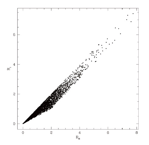
In Fig. 3, as an example, we show the observed daily number of sunspots (R_B) and R_i for a whole period assuming the exponential random noise with α = 0.1. We attempt to apply the linear least-squares method to the relationship between daily R_B and daily R_i to calculate the correction

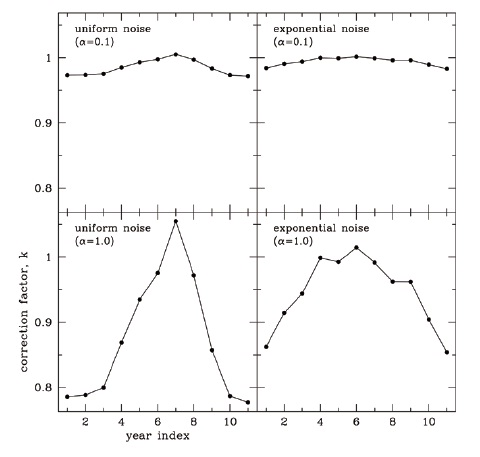
factor k_b in each year, after chopping the whole data set into 11 yearly data subsets. In Fig. 4, we show the resulting yearly k_b values as a function of years since the beginning of the solar cycle. Note that the scale is the same in every panel. Four cases of two random noise distributions with two different signal-to-noise ratios are indicated at the upper left corner in each panel. Resulting correction factors vary from year to year exactly, as was noticed by Oh & Chang (2012). That is, regardless of the noise distribution, we observe that the correction factor increases as the sunspot numbers increase. The typical uncertainties in determining the slope is the order of 0.01 and 0.001 for α = 1.0 and α = 0.1, respectively. These values are more or less the same for the exponential distribution and for the uniform distribution. The degree of the dependence is subject to the signal-to-noise ratio. Therefore, we consider that the apparent dependence of the value of correction factor k_b on the phase of the solar cycle is not due to a physical mechanism, but is a statistical property of the data. For instance, one may consider the dependence of the correction factor on the phase of the solar cycle since the numbers of large and small sunspots are different, so that the sensitivity, or the detectability of small sunspots, may be the cause of the dependence. If this is the case, as the solar cycle progresses, the size of sunspots could be considered as modulated, and as such the mechanism of sunspot formation under the solar surface is varying in time. What we show here is that this apparent dependence does not require such a complicated mechanism, but can be explained as a statistical property of the observed data. That is, a low number of sunspots results in a lower correlation coefficient in the R_B-R_i relationship. Furthermore, this effect turns out to be more serious when the noise level is high. When α is large, the resulting scatter (as shown in Fig. 1) gets broader, and as a result the least-squares fit is dominated by noise.

Monitoring sunspots regularly and consistently is an important and basic step in studying various aspects of solar activity. Observers must calculate their own correction factor k regularly and to keep it stable. In South Korea, sunspot observations have been performed at the Korea Astronomy and Space Science Institute (KASI) since 1987 (Sim et al. 1990, Kim et al. 2003) and at the ButterStar Observatory since 2002 (Oh & Chang 2012). All researchers have reported that revisions taking the yearly-basis k into account lead to results that agree better with R_i, and that yearly k apparently varies with the solar cycle. In this paper, using artificial data sets we have modeled, we attempt to investigate whether the variation in the correction factor is really coupled with the solar cycle. We have found that the apparent dependency is due to the statistical property of the data sets. Regardless of statistical distributions of the random noise, we observe the correction factor increases as the sunspot numbers increase. The degree of dependence is also subject to the signal-to-noise ratio. Therefore, we conclude that the apparent dependence of values of the correction factor k on the phase of the solar cycle is not due to a physical mechanism, but is a statistical property of the data.